In this post, I will explain the implementation of BRDFs for better material representation and I will explain using the object lights as light sources to finally move on to path tracing with Monte Carlo Integration. After that, I will explain several optimization techniques to make path tracing converge faster, such as Importance Sampling, Next Event Estimation and Russian Roulette.
BRDFs
BRDFs are an important part of the ray tracing pipeline and rendering equation, as they define how light interacts with the surfaces. The BRDFs are defined as the ratio of the outgoing radiance to the incoming radiance, and they are dependent on the incoming and outgoing directions of the light. In this implementation, I used Bling-Phong, Phong and Torrance-Sparrow BRDFs.

Rendering equation with BRDF part hightlighted
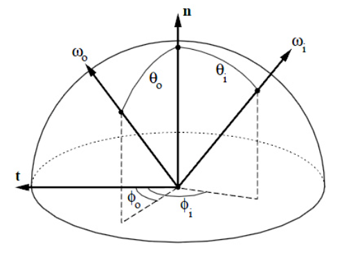
BRDF hemisphere representation, each different BRDF introduces different distribution on the surface
When we move into the path tracing, we need to be sure that the integral of the BRDFs around the hemisphere is equal to 1.0, as the BRDFs are defined as the ratio of the outgoing radiance to the incoming radiance. This is important as we need to sample the directions around the hemisphere, and the sum of the probabilities of the directions should be equal to 1.0. Because if we exceed this value, as we increase the sample number with the Monte Carlo Integration, we can’t converge to the correct value.
In the normal versions of the Bling Phong and the Phong BRDF there is a cosine variable at the denominator, however this prevents the BRDFs to be normalized, as the integral of the BRDFs around the hemisphere should be equal to 1.0. To fix this, we can use the modified versions of these BRDFs, which can be normalized.

Bling Phong BRDF equation
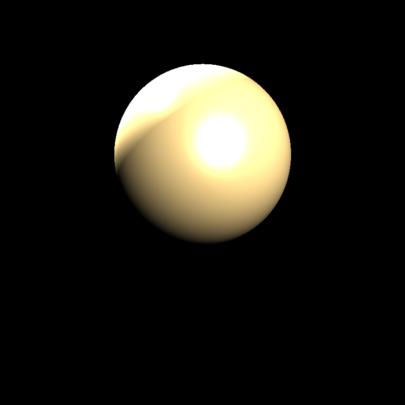
Bling Phong BRDF sphere

Modified Bling Phong BRDF equation
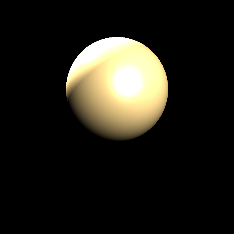
Modified Bling Phong BRDF sphere

Normalized Modified Bling Phong BRDF equation
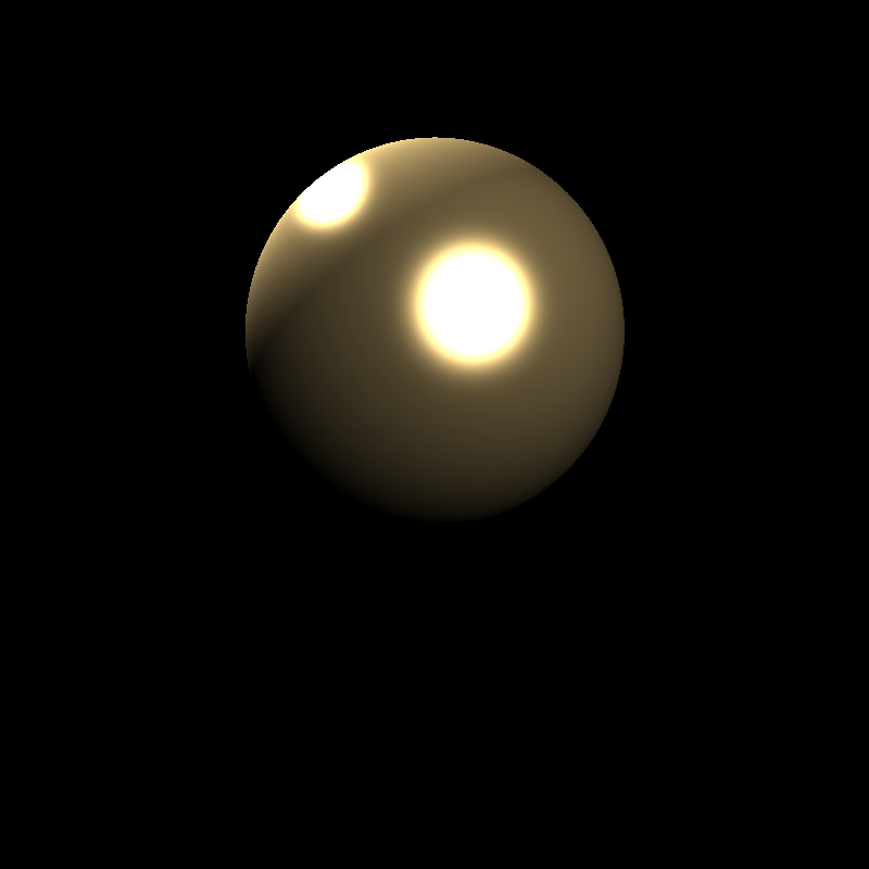
Normalized Modified Bling Phong BRDF sphere
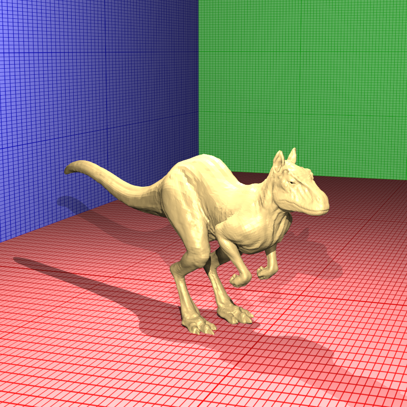
Killeroo model with Bling Phong BRDF

Phong BRDF equation

Phong BRDF sphere

Modified Phong BRDF equation

Modified Phong BRDF sphere

Normalized Modified Phong BRDF equation
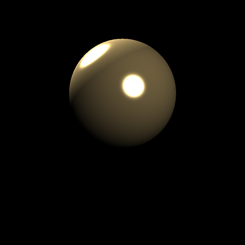
Normalized Modified Phong BRDF sphere

Torrance-Sparrow BRDF equation, F term is the Fresnel reflection term, D term is the micro-facet distribution term, G term comes from the shadowing and masking from the micro-facets
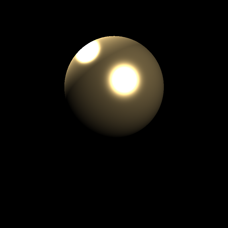
Torrance-Sparrow BRDF sphere
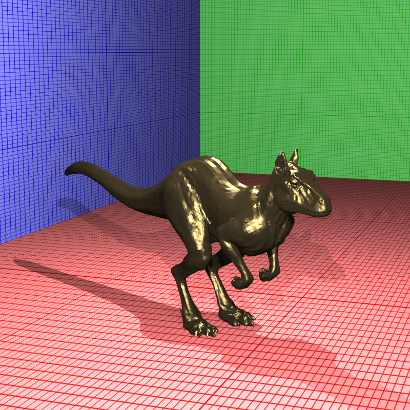
Killeroo model with Torrance-Sparrow BRDF
Object Lights
Another thing we need to worry when we move to the path tracing is lights, until now we used point lights, or directional lights as light sources, but in path tracing we need to hit these emissive objects to get the light. So we need lights with surfaces or meshes to emit light. To implement this, I created an another type of material called Emissive material, which emits light from the surface. This way, we can use any object as a light source, and we can move into the world of path tracing.
Sampling Points From Light Meshes
We need to introduce a cumulative distribution function (CDF) to sample points from the light meshes, as we need to sample points from the light meshes with respect to the area of the triangles. To do this, we need to calculate the area of the light meshes triangles, and create a CDF from the area values. After that, we can sample a random point from the light meshes with respect to the CDF values. To find the triangle that the CDF value corresponds to, we can use binary search, as the CDF values are sorted, however in my implementation I didn’t use binary search, as I used a simple for loop to find the triangle that the CDF value corresponds to because of the size of the light meshes.
triangleAreasCDF.resize(triangles.size());
for (uint32_t i = 0; i < triangles.size(); i++)
{
  triangleAreasCDF[i] = 0.0f;
  for (uint32_t j = 0; j <= i; j++)
    triangleAreasCDF[i] += triangleAreas[j];
  triangleAreasCDF[i] /= totalArea;
}

//sampling triangle
float r = frandom();
uint32_t idx = 0;
for (uint32_t i = 0; i < bvh->triangleAreasCDF.size(); i++)
{
  if (r < bvh->triangleAreasCDF[i])
  {
    idx = i;
    break;
  }
}

//sampling point from triangle
const triangle& tri = bvh->triangles[idx];
float r1 = frandom();
float r2 = frandom();

float sqrt_r1 = sqrt(r1);

return tri.p1 * (1.0f - sqrt_r1) + tri.p2 * (sqrt_r1 * (1.0f - r2)) + tri.p3 * (sqrt_r1 * r2);
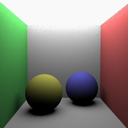
Cornell box with a mesh light
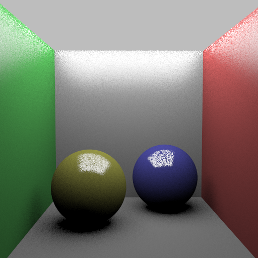
Cornell box with a mesh light, spheres with glossy surfaces
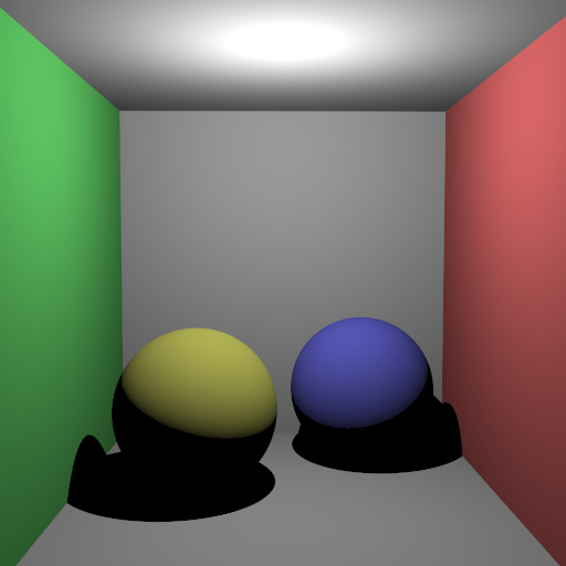
Cornell box with a point light for comparision, materials are not glossy
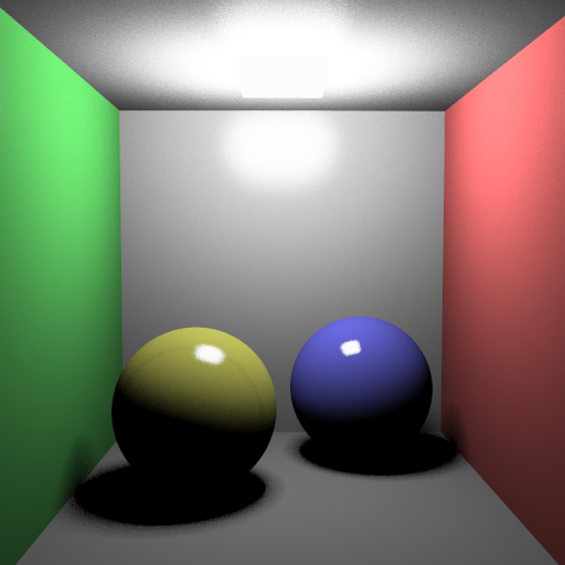
Cornell box with a small mesh light, spheres with glossy surfaces
Sampling Points From Light Spheres
To sample from sphere lights, we can act a little bit smarter and we can sample from the point which are visible to the intersection point, we can find the maximum angle with the vector from the center of the sphere to the interscetion point, which will be the tangent of the sphere from the intersection point. After that we can create a orthogonal basis with the normal of the intersection point, and the vector from the center of the sphere to the intersection point, and we can sample a random point from the sphere with respect to the maximum tangent angle.
float sin_theta_max = radius / glm::length(intersection - center);
float cos_theta_max = std::sqrt(std::max(0.0f, 1.0f - sin_theta_max * sin_theta_max));

//create a basis and sample a position
vec3 wtheta = glm::normalize(center - intersection);
vec3 np = create_non_colinear_vector(wtheta);
vec3 u = glm::normalize(cross(wtheta, np));
vec3 v = glm::normalize(cross(wtheta, u));

float ch1 = frandom();
float ch2 = frandom();

float theta = std::acos(1.0f - ch1 + ch1 * cos_theta_max);
float phi = 2.0f * pi * ch2;

vec3 l = glm::normalize(u * std::cos(phi) * std::sin(theta) + v * std::sin(phi) * std::sin(theta) + wtheta * std::cos(theta));
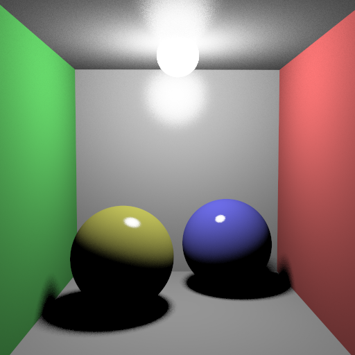
Cornell box with a sphere light, spheres with glossy surfaces
If we apply transformations to the sphere lights, we can create different light sources, like ellipsoids, or other shapes. This way we can create more complex light sources with simple shapes.
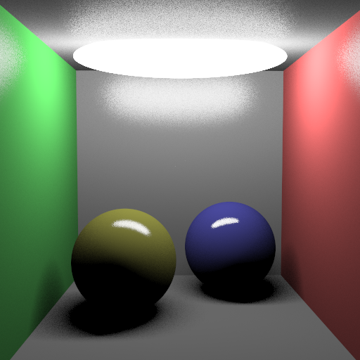
Cornell box with an ellipsoid light, spheres with glossy surfaces
Path Tracing With Monte Carlo Integration
To solve the rendering equation, we can use the Monte Carlo Integration, which is a simple way to estimate the integral of the rendering equation. We can sample the directions around the hemisphere, and we can calculate the radiance values for each sample, and we can average the radiance values to get the final radiance value. This way we can estimate the integral of the rendering equation, and we can get the final image. A thing to note is that we need to divide each sample with the probability of the sample, as we are using the Monte Carlo Integration, and we need to divide the sum of the samples with the sum of the probabilities of the samples to get the correct value. As the sample number increases, the radiance values will converge to the correct value, and we can get the final image.
The main difference in the implementation is that we need to indirect rays even with the diffuse surfaces, as in real life light bounces around all the surfaces, but with the rough surfaces light can bounce in different directions, so we need to sample the directions around the hemisphere, and we need to calculate the radiance values for each sample.
As a start we will use uniform sampling as we used in the environmental spherical lights, and like before we will take average of the radiance values to get the final radiance value.
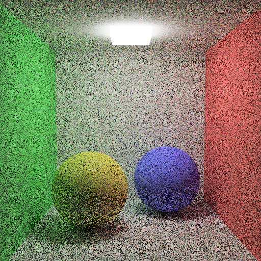
Cornell box with a prism light, 100 samples
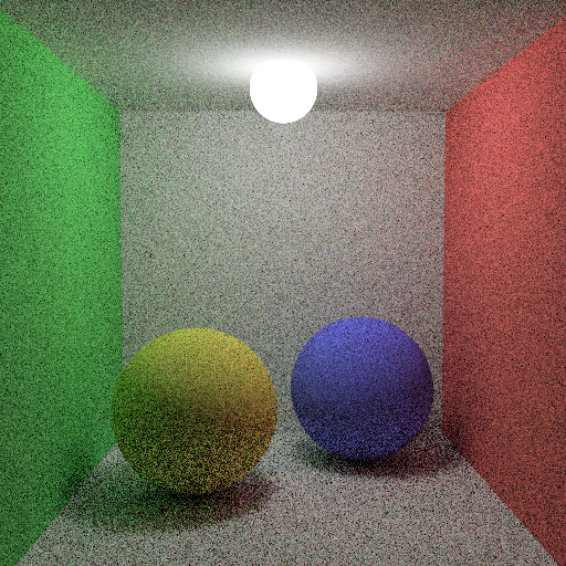
Cornell box with a sphere light, 400 samples
As you can see, the images are noisy, and we need to increase the sample number to get a less noisy image, but this will increase the rendering time, and we need to optimize the path tracing to get a less noisy image with less sample number.
Importance Sampling
Importance sampling means that we need to sample directions with the most of the radiance is concentrated. To do this we need to sample from the locations where lights are present or where the BRDFs are concentrated, or with an even simpler approach we can use the cosine weighted sampling. This cosine value comes from the term of the rendering equation, and it effects the total radiance comes from a certain angle with addition to other terms like BRDFs.

Cosine weighted sampling
To implement cosine sampling we need to build an orthogonal basis with the normal of the intersection point, and we need to sample a random point from the hemisphere with respect to the cosine value. Which means that we will be taking more samples from the directions where the cosine value is higher, and we will be taking less samples from the directions where the cosine value is lower. And after calculating the radiance coming from the sample we need to divide the radiance value with the cosine value divided by pi, which is the probability of the sample.
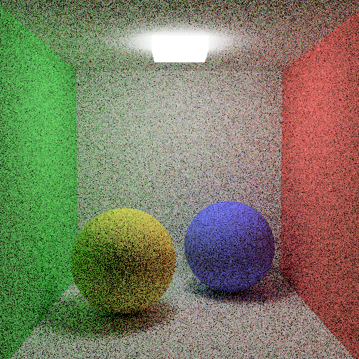
Cornell box with a prism light, 100 samples, importance sampling

Cornell box with a sphere light, 400 samples, importance sampling
As you can see, the images are less noisy, however not all the noise is gone but this indicates we are on the right track.
Next Event Estimation
We need to sample from the directions with the most contribition to the radiance, how about sampling from the light sources directly? This is the main idea behind the Next Event Estimation, in each indirect ray we can sample from the light sources directly, and we can calculate the radiance values for each sample. This way we can get the most contribution to the radiance, and we can get a less noisy image with less sample number. This technique doesn’t introduce any bias to the image, because when we sample from the light sources directly, we treat them like any other ray we sampled randomly.

Cornell box with a prism light, 100 samples, Next Event Estimation
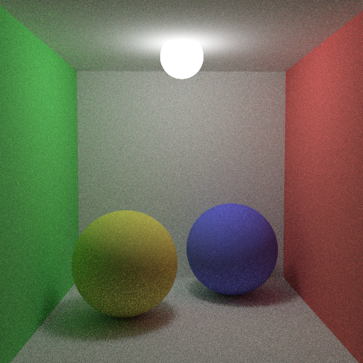
Cornell box with a sphere light, 400 samples, Next Event Estimation
As seen in the images, the noise are far less, however we introduced new kind of noise which is called fireflies, these are the bright pixels in the image, and they are caused by the direct sampling from the light sources, and they are hard to get rid of.
Wrong Implementation With Less Noisy Result
While implementing the Next Event Estimation, I was tinkering with the BRDFs and mesh light equations, and in one try, I didn’t normalized the wi (light vector) and calculated the cosine values with this unnormalized vector, and I got a way less noisy result with the same number of samples. I didn’t quite understand the reasoning behind this, I just wanted to share this with you.
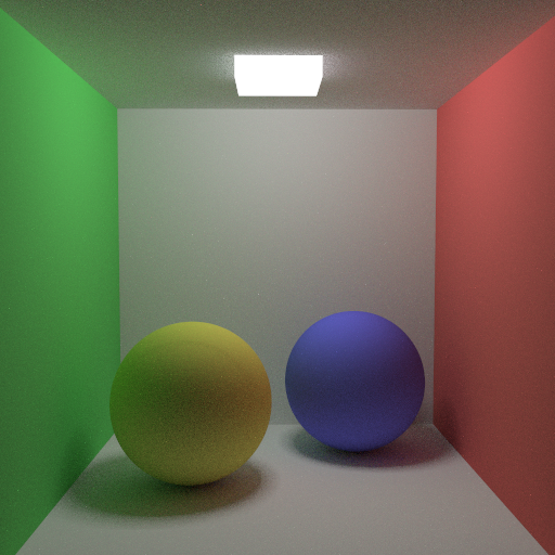
Cornell box with a sphere light, 100 samples, Importance Sampling, Next Event Estimation, Wrong Calculation

Cornell box with a sphere light, 100 samples, Importance Sampling, Next Event Estimation, Correct Calculation
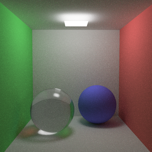
Cornell box with a sphere light, 400 samples, Importance Sampling, Next Event Estimation, Correct Calculation, Glass Material
Splitting
While sampling multiple rays from one pixel, we can use another kind of parameter to multiply the samples, which is called splitting. We can split the samples with a certain number from each intersection. This can help us to sample from the intersection points with more samples, and we can sample from where it is important to the final image.
Russian Roulette
Russian Roulette is a technique to terminate the rays with a certain probability, this way we can reduce the number of samples and we can get a less noisy image with less sample number. We can terminate the rays with a certain probability, and we can multiply the radiance values with the inverse of the probability, this way we can get the correct radiance values. While implementing this I used the maximum component of the diffuse and speculer reflectance values, I didn’t use the length of these values, because if a materials red reflectance is 1.0, it will be an important ray to our image, even if the other components are 0.0. I killed rays before the splitting happens because with this way I get faster and more accurate results.

Cornell box with a sphere light, 25 samples, Importance Sampling, Next Event Estimation, Russian Roulette, Rays Splitting into 2
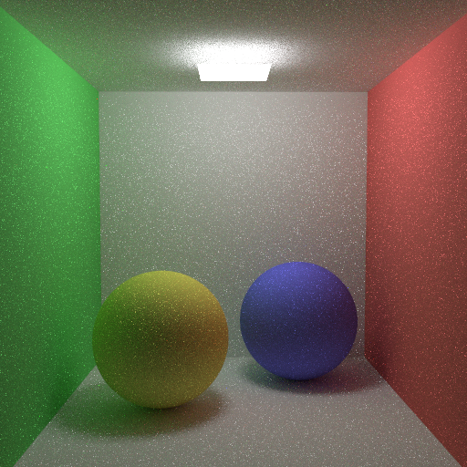
Cornell box with a sphere light, 25 samples, Importance Sampling, Next Event Estimation, Russian Roulette, Rays Splitting into 3
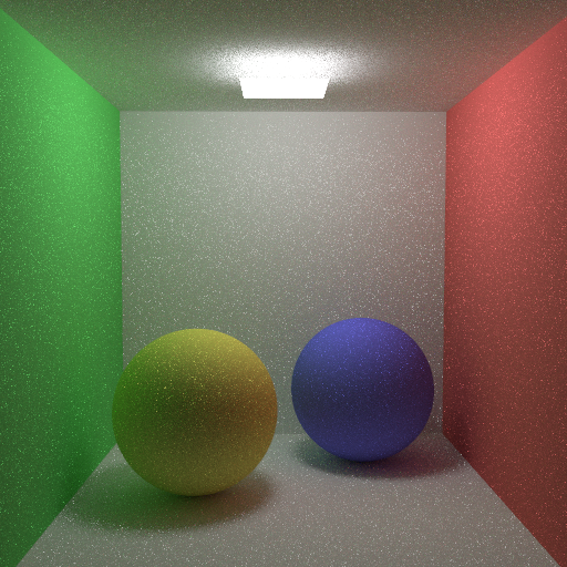
Cornell box with a sphere light, 25 samples, Importance Sampling, Next Event Estimation, Russian Roulette, Rays Splitting into 4
These results are far less noisy from the point that we are started, and looking realistic with all the color blendings and soft shadows.
Bloopers
While implementing the path tracing, I encountered several problems producing some fun results, I wanted to share them with you.
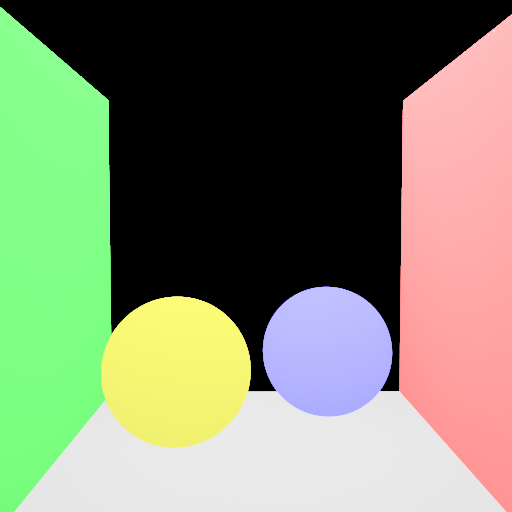
We converged a little bit early
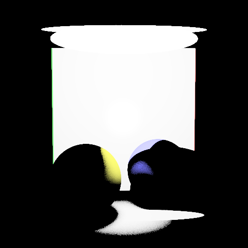
Like an alien abduction
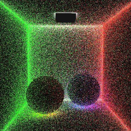
Some neon vibes
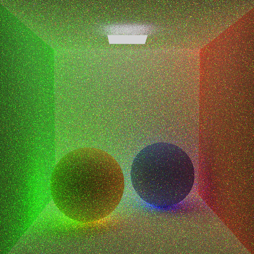
Neon vibes, but brighter
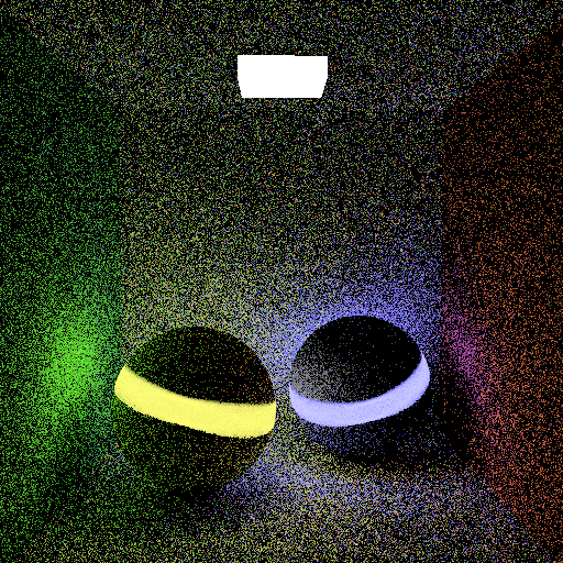
Like the movie Tron
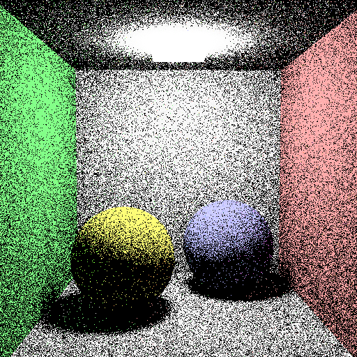
Could it be an cartoon shader?
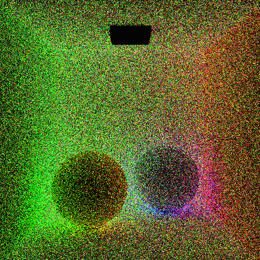
Lost in the noise
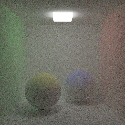
Fogs without additional cost
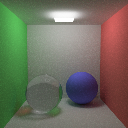
Light mesh in the glass seems suspicious
Future Work
My main plan is to move these implementations on a GPU path tracer with DXR. In the end, I want to implement a path tracing suit with preview GPU renderer and a CPU renderer with more functionalities like volumetric rendering, Disney BRDFs, subsurface scattering, and more. Stay tuned for the next posts.
References
Ahmet Oğuz Akyüz, Lecture Slides from CENG795 Advanced Ray Tracing, Middle East Technical University