In this post, I will explain the implementation of spot, directional and environmental lighting. As for environmental lighting, I will explain how to use an HDR image as a light source. In the end, I will show how to implement tonemapping to properly display the final image.

Spot Light

After implementing point lights, spot lights can achieve a realisctic lighting effect without much effort. The only difference between a point light and a spot light is that spot light only lights an area in a direction, we can apply it to the equations by a direction vector and a cutoff and falloff angle. The intensity of the light will be calculated by the angle between the direction vector and the vector from the light source to the point, with respect to the cutoff and falloff angles.

color get_intensity(vec3 wi) const override
{
  float angle = glm::acos(glm::dot(glm::normalize(direction), glm::normalize(-wi)));

  if (angle > coverage)
    return color(0.0f);
  else if (angle < falloff)
    return intensity;
  else
  {
    float d = glm::cos(angle) - glm::cos(coverage);
    float n = glm::cos(falloff) - glm::cos(coverage);
    float s = powf(d/n, 4.0f);
    return intensity * s;
  }
}

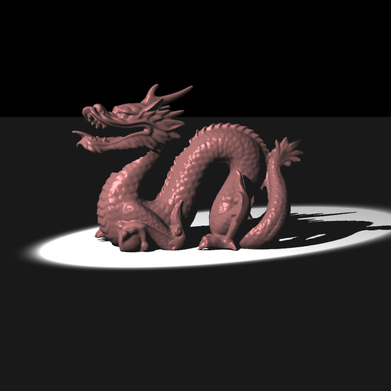
Dragon model with a spot light

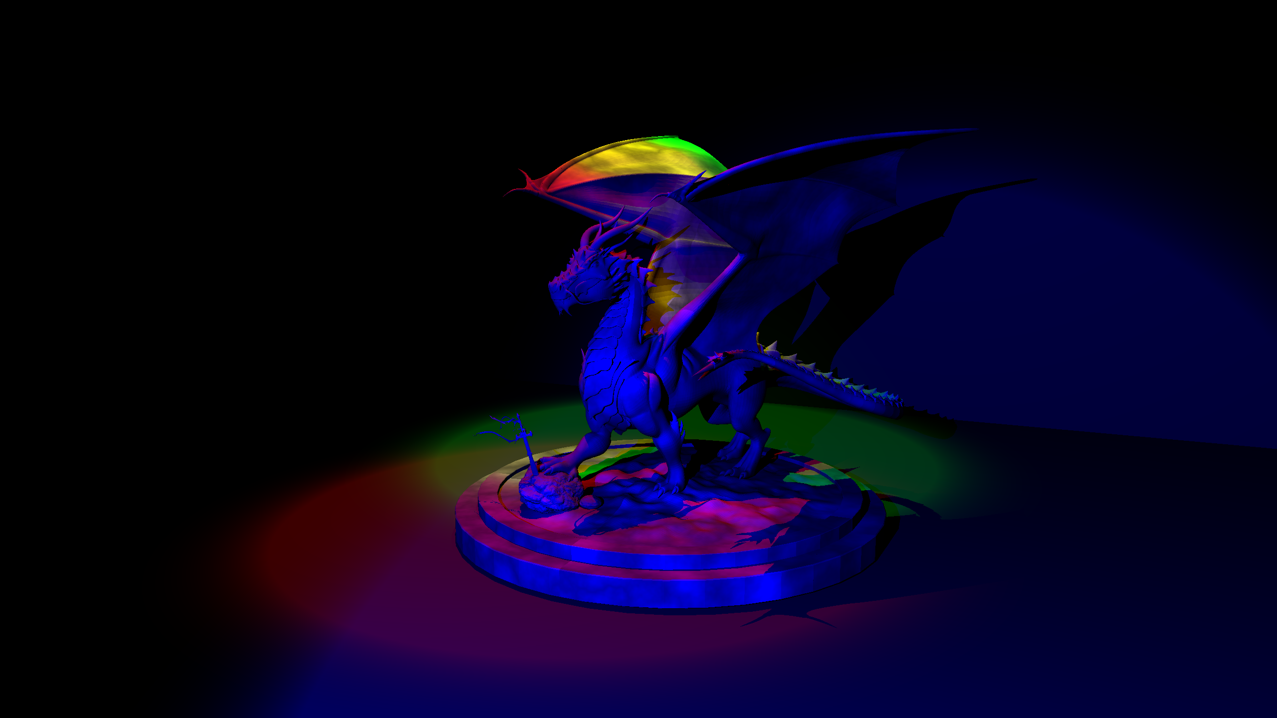
Different dragon model with tree spot lights

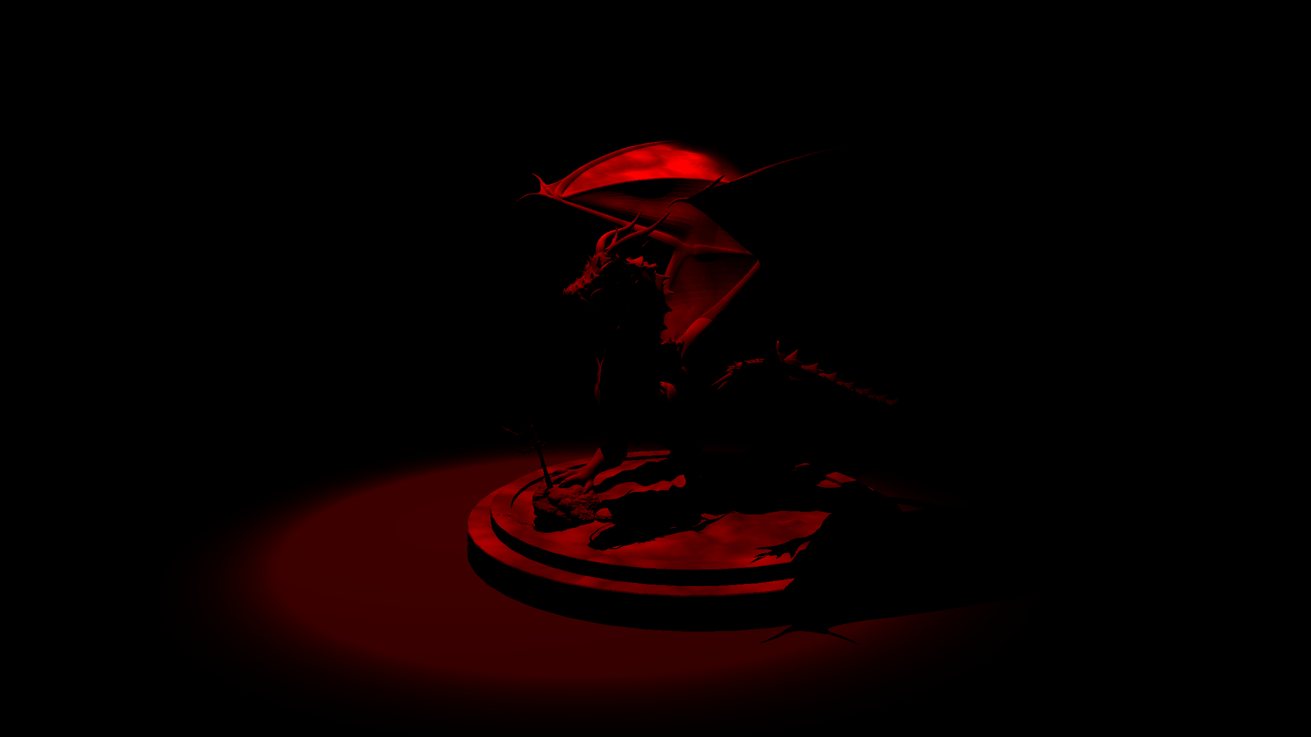
Same scene with a parser error, making it a bit scarier

Directional Light

Directional light is even simpler to implement, as it is a light source that is infinitely far away, and has a constant direction. This can be used to simulate sunlight, or any other light source that is far away from the scene. The intensity of the light is constant, and the direction is the same for all points in the scene.

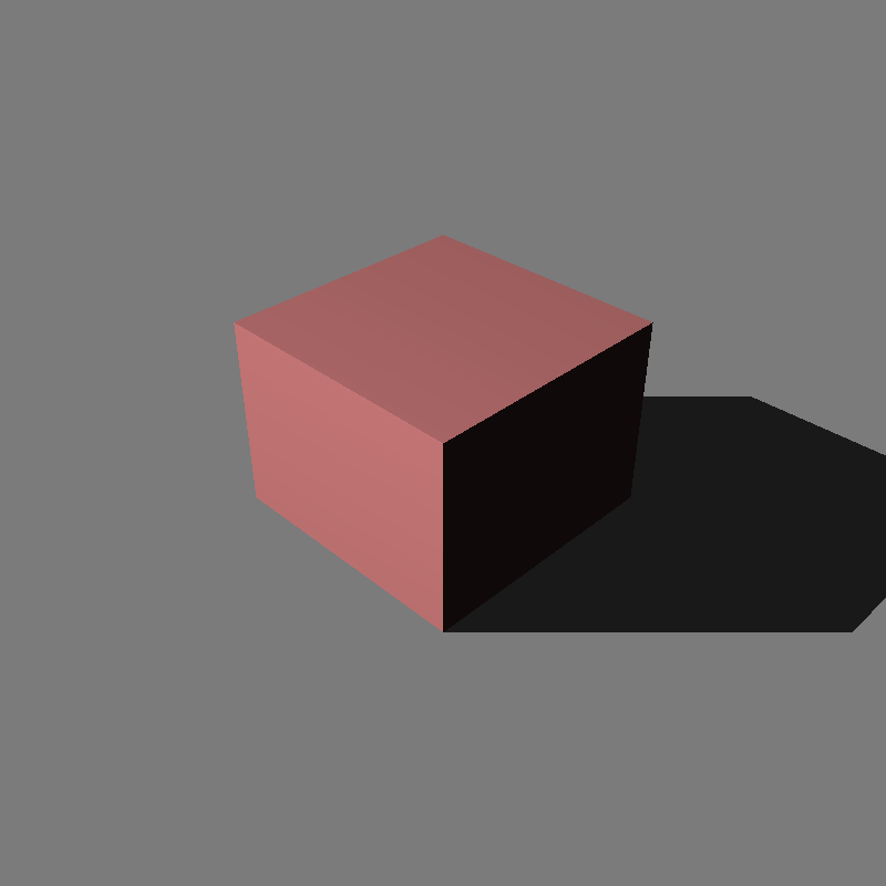
Cube with a directional light present

Spherical Directional Light (as Environmental Light)

We can think of environmental lights as spheres that encase the scene, and emit light from all directions. This can be used to simulate the light coming from the sky, or any light present in the environmental map. The intensity that we get from the environmental map image needs to present a more wide range of values than the other light sources, as it is a light source that is present in all directions, as there are non-light sources will be present in these images. To properly mimic these spherical directional lights we can use HDR images, which have a higher range of values than the usual 0-1 range. The light sources in these images will be greater than 1.0.

We will use two types of environmental maps, one is a simple image that is mapped to a sphere, and the other is a latidude-longitude map.

Latidude-Longitude Mapping (Panaromic)

From the direction we can calculate the UV coordinates of the image, like the code snippet below. This is also known as an equirectangular mapping, it maps the direction’s azimuth to the horizontal coordinate and its elevation to the vertical coordinate of the image.

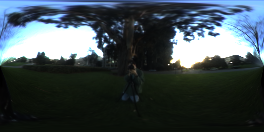
Latidude-Longitude Map

vec3 dir = generateUpperHemisphereVector();
float u = (1.0f + (atan2(dir.x, -dir.z) / pi) ) / 2.0f;
float v = acos(dir.y) / pi;

color c = env_texture->value(u, v, dir) * 2.0f * pi;
out_direction = dir;
out_intensity = c;

Spherical Mapping

The other type of environmental map is a simple image that is mapped to a sphere. The center of image corresponds to the forward (-z) direction, and the circumference is the backward (+z) direction. The horizontal line linearly maps the azimuthal angle to the pixel coordinate.

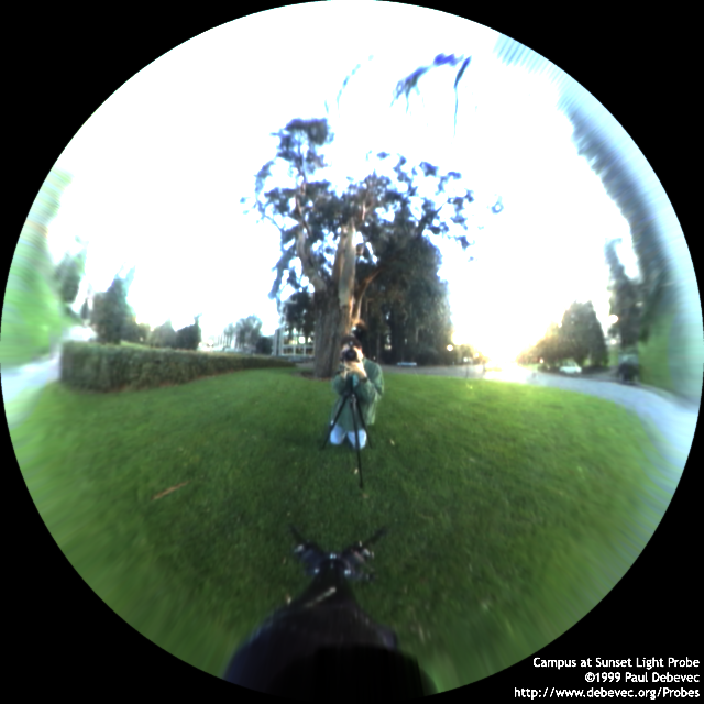
Spherical Map

vec3 dir = generateUpperHemisphereVector();
float r = (1.0f / pi) * ((acos(-dir.z) / sqrtf(dir.x * dir.x + dir.y * dir.y)));
float u = (r * dir.x + 1) / 2.0f;
float v = (r * -dir.y + 1) / 2.0f;

color c = env_texture->value(u, v, dir) * 2.0f * pi;
out_direction = dir;
out_intensity = c;

Sampling Directions with Rejection Sampling and Bugs

To sample from these images, we need a direction vector as we treat this images as the spheres. We can use rejection sampling in order to get a random direction in the upper hemisphere. While implementing this part I encountered a problem with my sampling code, when I sample a direction from a intersection point I always take the upper hemisphere as the unit spheres, +z part. This caused images being darker than they should be on the edges, and faces pointing below. After some time trying to find a magical eqauations which increases the brightness as the angle between the view direction and the normal increases, I realized that I was sampling the wrong hemisphere. I should adjust the angle of the hemisphere with the normal vector of the intersection point. Which is easy to do with the rejection sampling, as we can just sample a random direction and check if it’s dot product with the normal is positive or not.

vec3 dir = generaterRandomUnitVector();
while (dot(dir, normal) < 0.0f)
{
  dir = generaterRandomUnitVector();
}

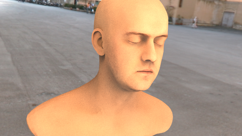
Lights sampled with wrong directions, faces near the object outlines appear darker

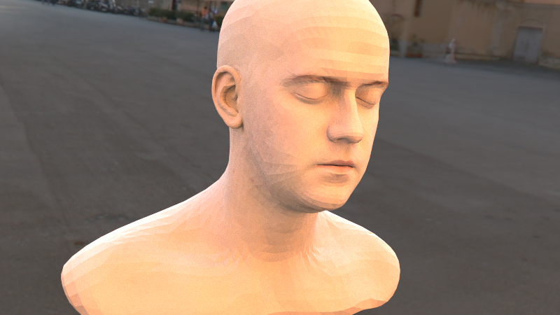
Lights sampled with correct directions

Color Adjustments for HDR Rendering

Until now, the code worked on the 0.0f-255.0f range, as to mimic the 8bit color range calculations on the pipeline, and in the end the values are clamped. After the HDR mapping implementations, the color values can be larger than the floating point’s precision limits (>1m), which causes problems. To fix this, I adjusted the code to work in the 0.0f-1.0f range as default range, and HDR range extends this range. This way, the calculations will be more precise and the final image will be more accurate.

Tonemapping (Photographic TMO)

To display the final image, we need to apply some tonemapping calculations to display HDR range properly, as the monitors can only display a limited range of values. The most common tonemapping algorithm is Reinhard’s tonemapping operator, which is a simple and effective way to display HDR images.

At the first part of this algorithm, we map the luminance range of the image to the 0.0f-1.0f range, by calculating the average luminance of the image. The most used default key for this mapping is 0.18f, which is mapped to the middle gray value (log-average-luminance) on image.

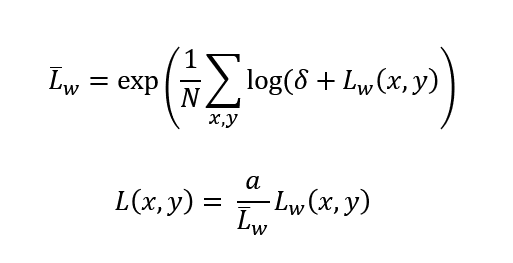
After the first step, we will compress the luminance values with sigmoidal compression, and we can apply a burnout effect to the bright areas of the image.

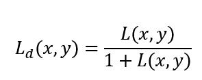
Sigmoidal compresiion

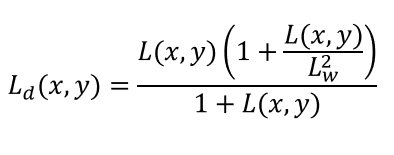
Compression with burnout values

In the end to display images in .png format (LDR), we need to convert the values back to 0-255 range, and clamp the values to this range.

Compression with burnout values

Final code is like as below:

int pixel_count = imageWidth * imageHeight;
float epsilon = 1e-5;

std::vector<float> luminance_values;
luminance_values.reserve(pixel_count);
float total_log_luminance = 0.0f;
for (int j = imageHeight - 1; j >= 0; j--)
{
  for (int i = 0; i < imageWidth; i++)
  {
    color c = img[j][i];
    float luminance_world = luminance(c);
    total_log_luminance += log(epsilon + luminance_world);
  }
}

float lwp = exp((1.0f / pixel_count) * total_log_luminance);

for (int j = imageHeight - 1; j >= 0; j--)
{
  for (int i = 0; i < imageWidth; i++)
  {
    color c = img[j][i];
    float l = (scene_cam.key_value / lwp) * luminance(c);
    luminance_values.push_back(l);
  }
}

std::sort(luminance_values.begin(), luminance_values.end());

//get the burnout percentage
float burnout_percentage = scene_cam.burn_percent / 100.0f;
float lwhite = 0.0f;
if (scene_cam.burn_percent != 0.0f)
{
  int burnout_index = (int)(pixel_count * (1.0f - burnout_percentage));
  lwhite = luminance_values[burnout_index];
}

for (int j = imageHeight - 1; j >= 0; j--)
{
  for (int i = 0; i < imageWidth; i++)
  {
    color& c = img[j][i];

    float ld = 1.0f;
    if(scene_cam.burn_percent != 0.0f)
    {
      //eq 4
      float l = (scene_cam.key_value / lwp) * luminance(c);
      ld = (l * (1.0f + (l / (lwhite * lwhite)))) / (1.0f + l);
    }
    else
    {
      float l = (scene_cam.key_value * luminance(c)) / lwp;
      ld = l / (l + 1.0f);
    }

    auto tmpc = c;
    if(luminance(c) < 0.00001f)
    {
      continue;
    }

    float lum = luminance(c);
    c.x = ld * (powf(c.x / lum, scene_cam.saturation));
    c.y = ld * (powf(c.y / lum, scene_cam.saturation));
    c.z = ld * (powf(c.z / lum, scene_cam.saturation));

  }
}

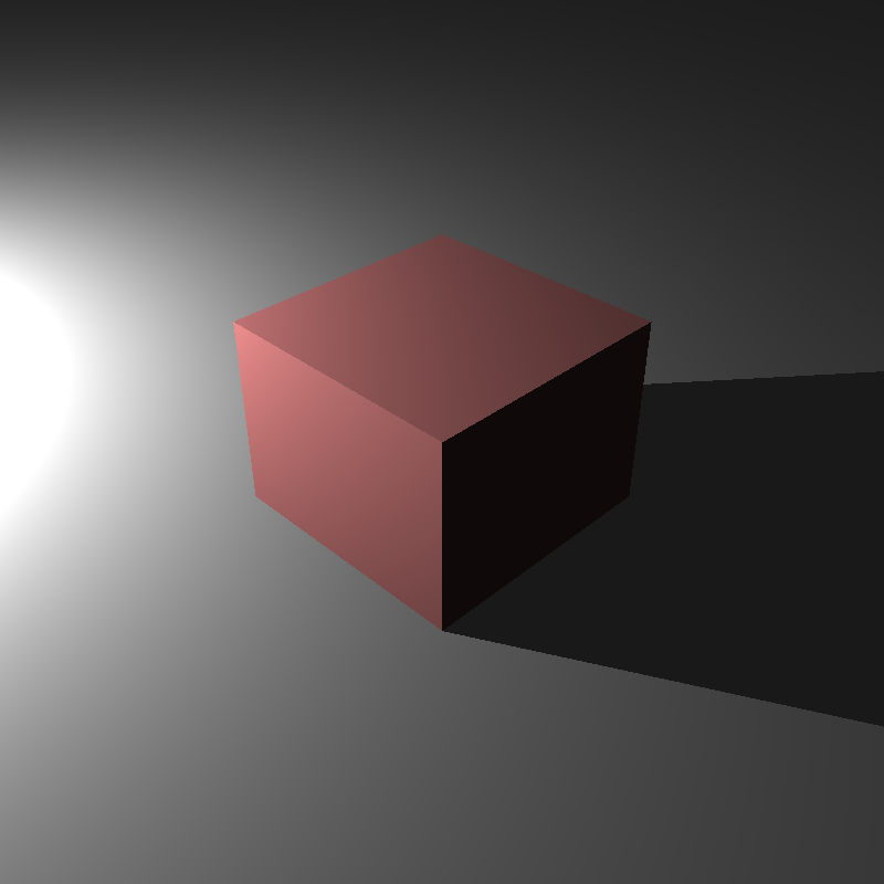
Cube and a point light without tonemapping

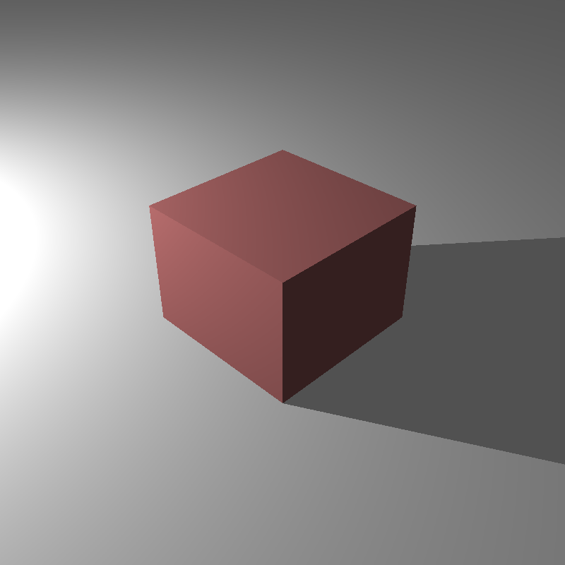
Cube and a point light with tonemapping

Negative UV values

While rendering final images, I encountered a problem with the UV values of the image, as the values were negative. This caused wrong textures on images, which I noticed after rendering a car model with 1600 samples in 1 hour. At first, I tried to clamp values, applyind modulo opearations, but none of them gave correct results, in the end the fix was simple, I just take the absolute value of the UV coordinates.

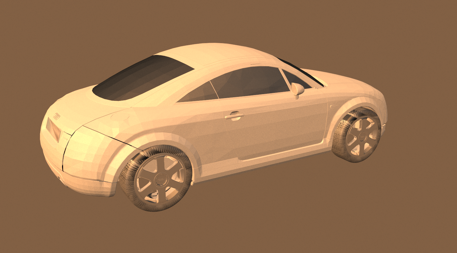
Car model with wrong texture coordinates and missing shadows

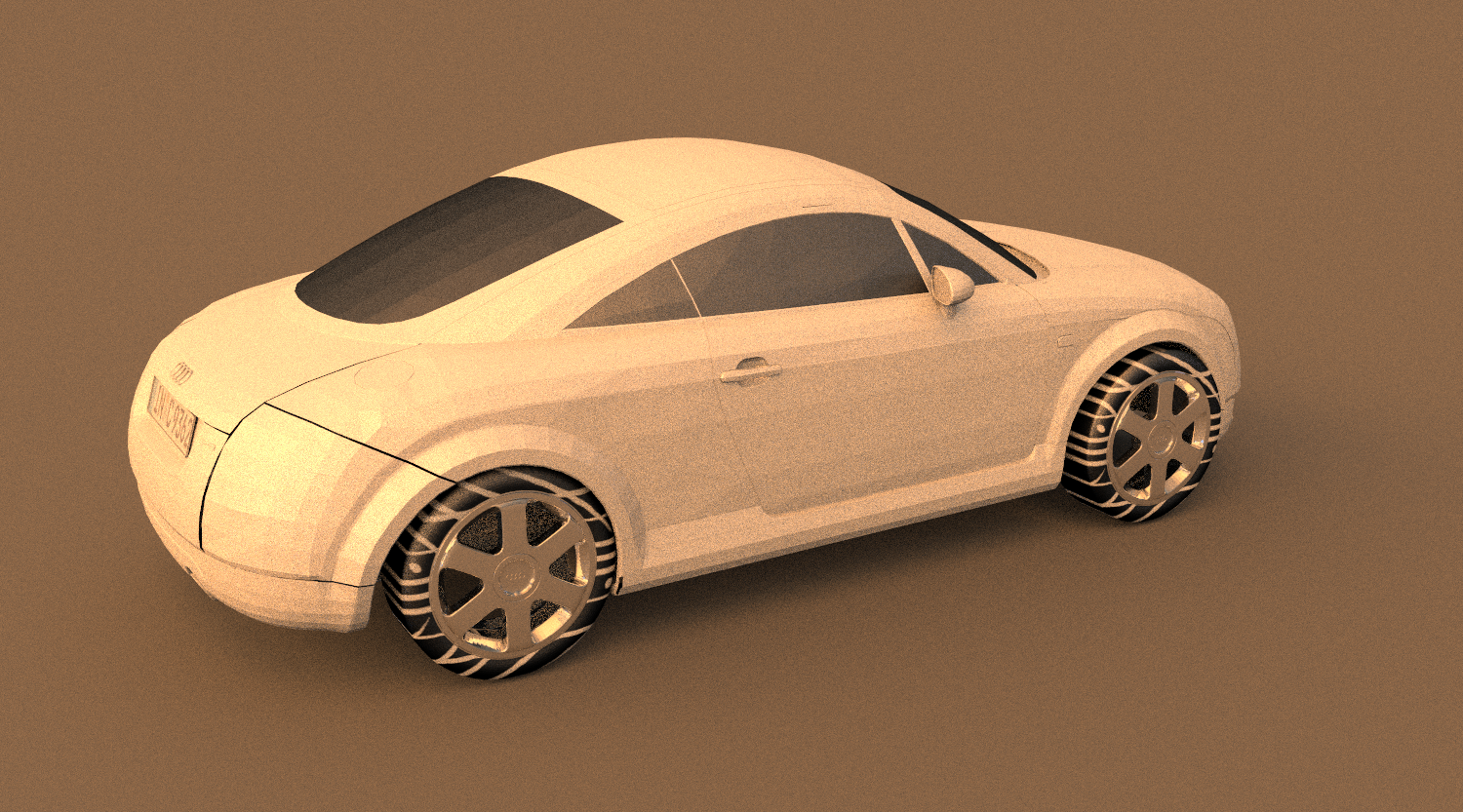
Car model with less samples but correct shadows and textures, we can see the soft shadows created by the multisampling with different directions

Results

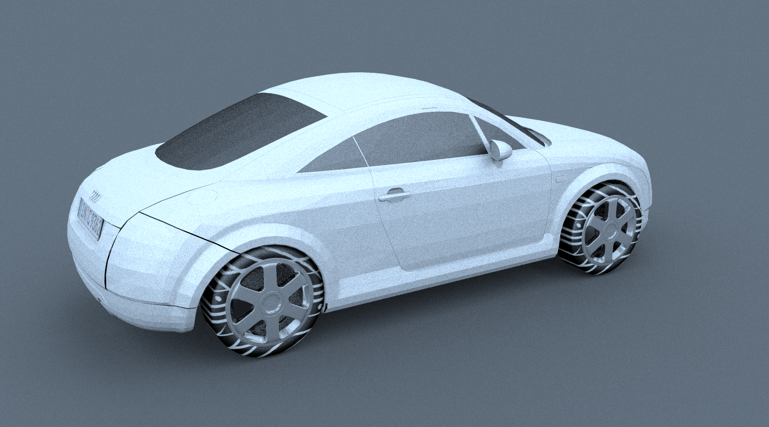
Car model with a different environmental map, the difference is huge

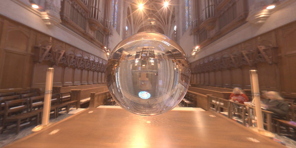
Glass sphere with an environmental map

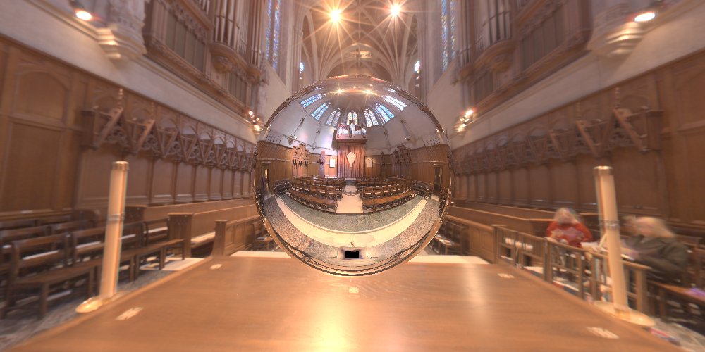
Mirror sphere with an environmental map

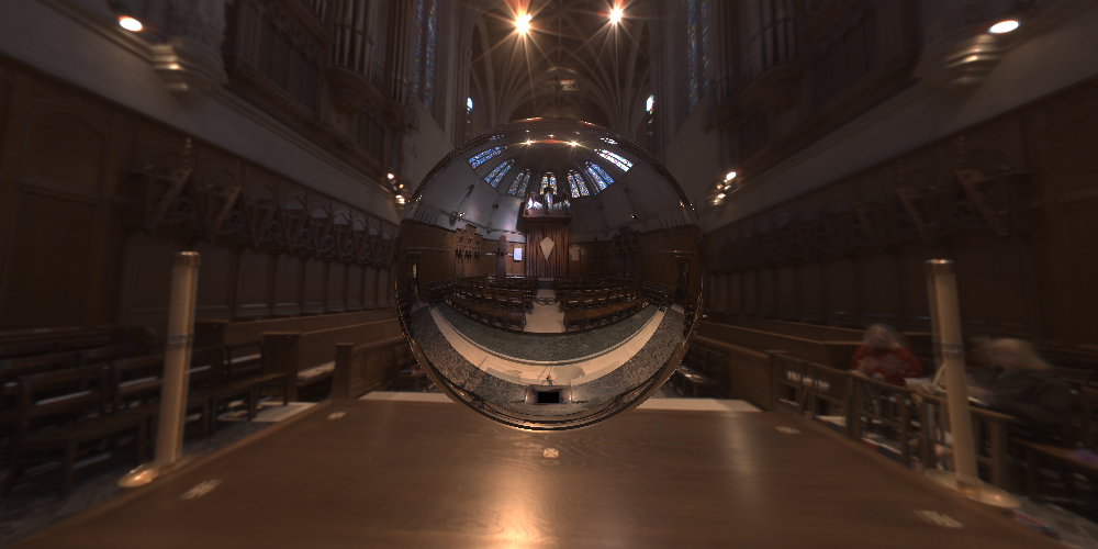
Mirror sphere with an environmental map without tonemapping

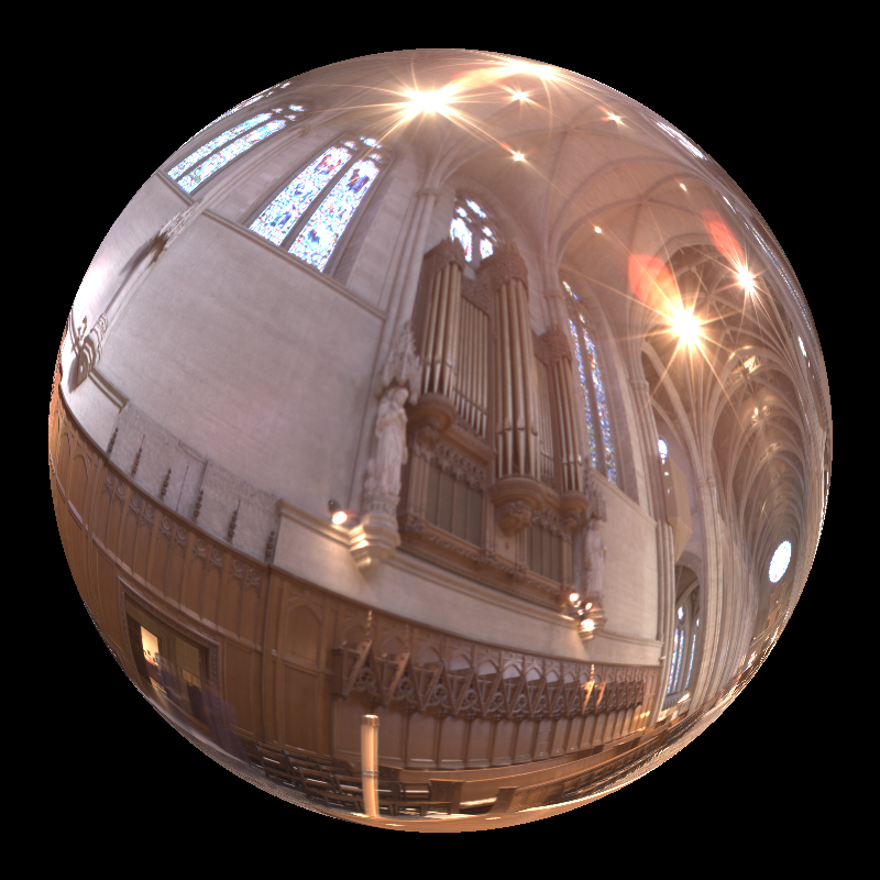
Sphere with a point light and an environmental map

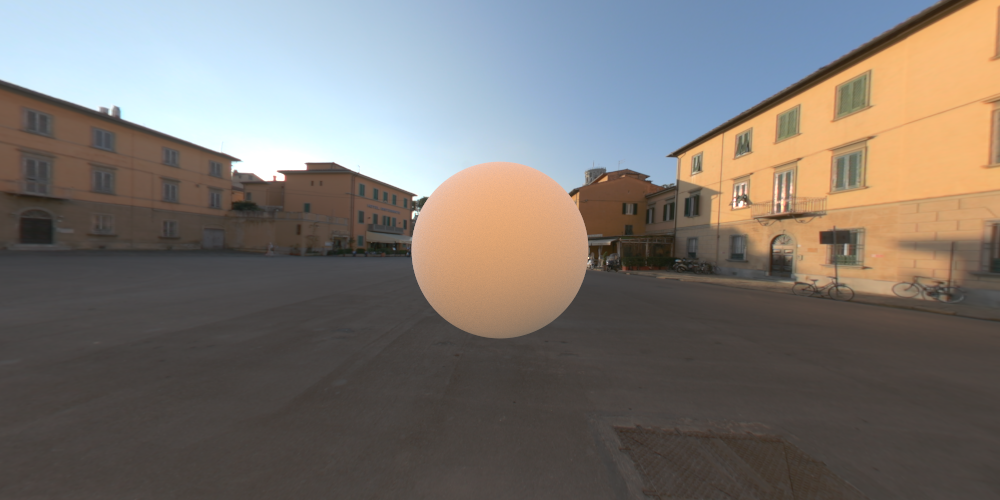
Sphere with an environmental map

References

Ahmet Oğuz Akyüz, Lecture Slides from CENG795 Advanced Ray Tracing, Middle East Technical University

Reinhard, E., Stark, M., Shirley, P., & Ferwerda, J. (2002, July). Photographic tone reproduction for digital images. In Proceedings of the 29th annual conference on Computer graphics and interactive techniques (pp. 267-276). https://web.tecgraf.puc-rio.br/~scuri/inf1378/pub/reinhard.pdf

High-Resolution Light Probe Image Gallery, https://vgl.ict.usc.edu/Data/HighResProbes/