In this post, I will explain the implemenation of texture sampling methods. After that I will explain how to implement normal mapping and bump mapping. In the end I will show how to create procedural textures with perlin noise, and will use these as bump maps.
Texture Sampling
To create a colorful model we can chane the materials of the triangles, or vertices and then interpolate them inside the triangle, however to create realistic looking models we just need more resolution. If we try to achieve this with triangles and vertices, we would need too much vertices that will slow our raytracer down. Instead we can sample the colors on our models from 2D images. To map 2D images into our model we will need to project our models into 2D plane, which is called “UV Unwrapping”, in the essence this process will lay all the triangles down to the 2D plane and gave each vertex a ssecondary coordinate with 2 values, u and v. After that we can sample the colors from the image with these coordinates. For triangle meshes when we intersect with a triangle, we can get the barycentric coordinates of the intersection point and use these to interpolate the u and v values of the intersection point. After that we can use these values to sample the color from the image.
//calculate barycentric coords, and interpolate uv
vec3 v0v1 = v1 - v0;
vec3 v0v2 = v2 - v0;
vec3 v0p = P - v0;

float d00 = dot(v0v1, v0v1);
float d01 = dot(v0v1, v0v2);
float d11 = dot(v0v2, v0v2);
float d20 = dot(v0p, v0v1);
float d21 = dot(v0p, v0v2);

float denom = d00 * d11 - d01 * d01;
float v = (d11 * d20 - d01 * d21) / denom;
float w = (d00 * d21 - d01 * d20) / denom;
float u = 1.0f - v - w;
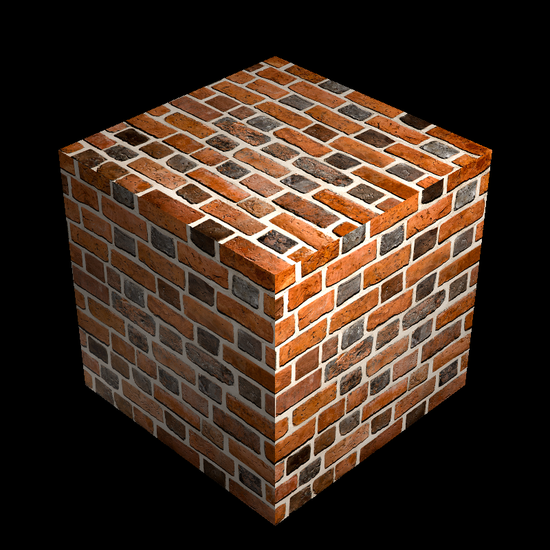
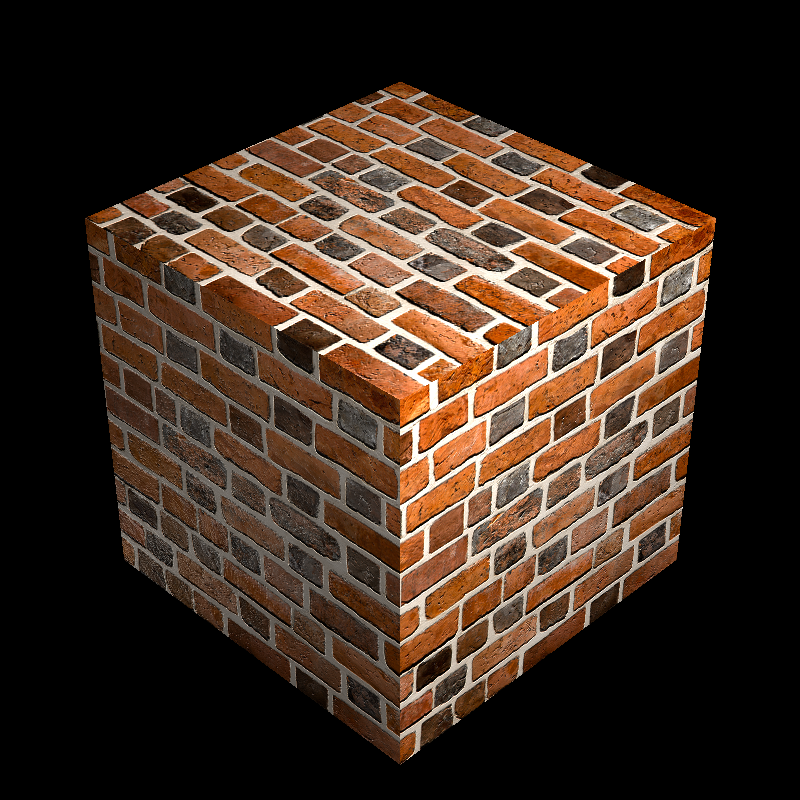
Brick wall texture mapped onto a cube, values replacing diffuse reflectance
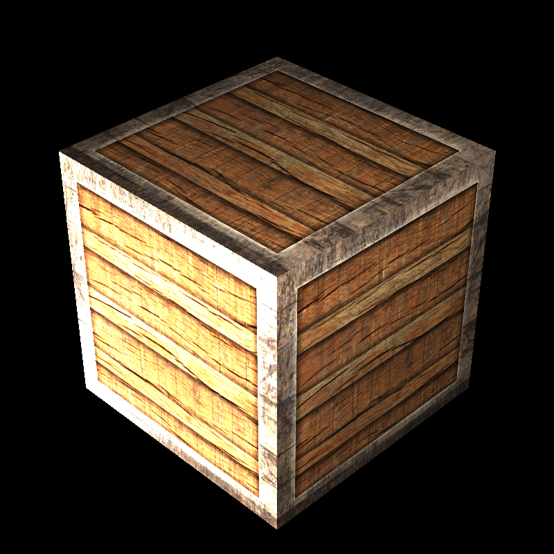
Wood texture mapped onto a cube, values replacing diffuse reflectance
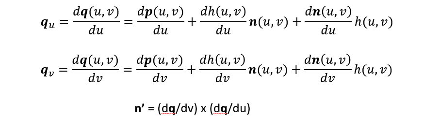
For the speres, we can use the spherical coordinates to map the texture onto the sphere. To do so we can use the following code snippet, which calculates the angles between the intersection point and the center of the sphere. After that we can use these angles to calculate the u and v values of the intersection point.
auto xyz = r.at(rec.t) - center;

auto theta = std::acos(xyz.y() / radius);
auto phi = std::atan2(xyz.z() , xyz.x());

rec.uv.e[0] = (-phi + pi) / (2 * pi);
rec.uv.e[1] = theta / pi;
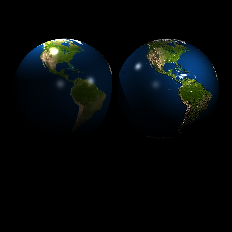
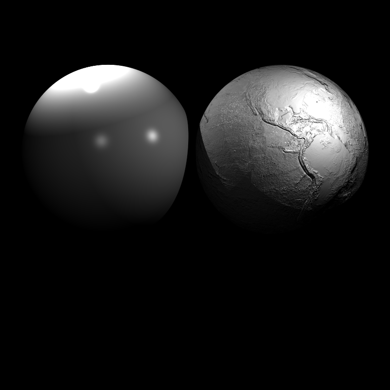
Earth texture mapped onto a sphere, left is a bumped version which I will cover later on
Nearest Neighbor Sampling vs Bilinear Sampling
To sample the colors from the image, we can use different methods, nearest neighbor will be the simplest one which will get the value of the nearest pixel on the image. However, this can create aliasing artifacts on the images with edges. To improve the situation we can just get sample from the nearest 4 pixels and interpolate the colors with the distance of the intersection point to the pixels. This method is called bilinear sampling.
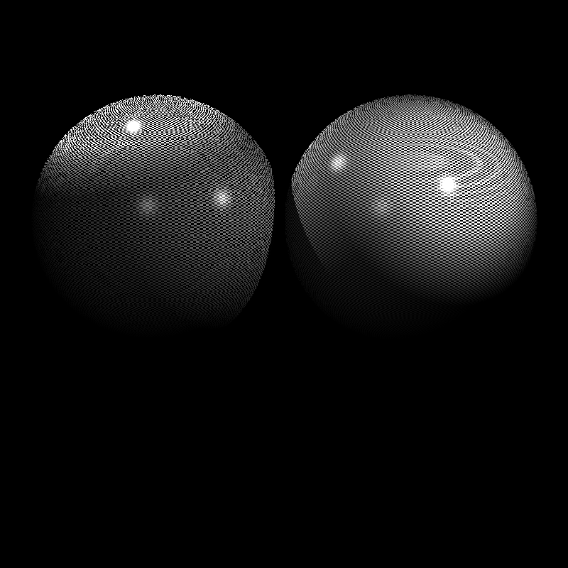
Nearest neighbor sampling vs bilinear sampling
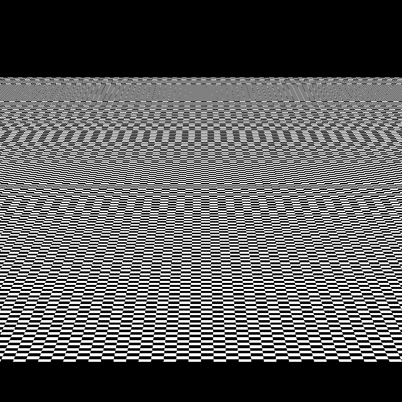
Nearest neighbor sampling
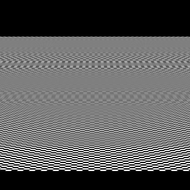
Bilinear sampling
Normal Mapping
We can get more detail from the textures besides the color values. We can use the normal values from the textures to create more detailed models. Which can create a visual effect of more detailed models without changing the geometry. However, we can’t just sample from the textures and use them as normals, because the normals can change with the transformation of the model. If we just use the world space normals from the textures, the normals will be wrong when the model is rotated or scaled. However, there is a fix for this, we can just define another space for the normals which remains unchanged when the model is transformed. This space is called the tangent space. To define the tangent space, we can just use the tangent and bitangent vectors of the model. The tangent vector is the vector that is perpendicular to the u axis of the UV coordinates, and the bitangent vector is the vector that is perpendicular to the v axis of the UV coordinates.
Tangents and Bitangents
At the begining, I thought if we have a normal map we can just use it on the every renderer and get same results. However, then I noticed that there are infinite number of tangents and bitangents for a intersection point on a mesh. To fix this problem, there are some methods, which the industry not quite agreed on. I found online that the MikkTSpace is the most popular one which aims to create a consistent tangent space for the models. It’s purpose is to create a tangent space which is consistent with the model’s geometry, importing order and such. However, we will not use this method for this post, and we will use the “dPdu” and “dPdv” vectors to calculate the tangent and bitangent vectors, which are the partial derivatives of the position vector with respect to the u and v values of the UV coordinates.
For triangles, we can use the following code snippet to calculate the tangent and bitangent vectors.
vec2 deltaUV1 = uv2 - uv1;
vec2 deltaUV2 = uv3 - uv1;
vec2 duv02 = uv1 - uv3, duv12 = uv2 - uv3;
vec3 dp02 = p1 - p3, dp12 = p2 - p3;
float determinant = duv02[0] * duv12[1] - duv02[1] * duv12[0];
if (determinant < 0.1f && determinant > -0.1f) {
      CoordinateSystem(unit(cross(p3 - p1, p2 - p1)), rec.dpdu, rec.dpdv);
} else {
  rec.tangent = (tv0v1 * deltaUV2.y() - tv0v2 * deltaUV1.y()) / (deltaUV1.x() * deltaUV2.y() - deltaUV1.y() * deltaUV2.x());
  rec.bitangent = (tv0v2 * deltaUV1.x() - tv0v1 * deltaUV2.x()) / (deltaUV1.x() * deltaUV2.y() - deltaUV1.y() * deltaUV2.x());
}
You can see the determinant check in the code snippet, this is to check if the triangle is degenerate or not. If the determinant is close to zero, the triangle is degenerate and needs to be handled differently. In this case, we can just use the cross product of the two edges of the triangle to get the normal of the triangle and use it to create a orthogonal basis for the tangent space.
For the spheres, we can use the following code snippet to calculate the tangent and bitangent vectors, which is the result of the mathematical derivation of the partial derivatives.
vec3 tangent, bitangent;
tangent = (vec3(2.0 * pi * xyz.z(), 0.0, -2.0 * pi *(xyz.x())));
bitangent = (vec3(pi * xyz.y() * cos(phi), -pi * radius * sin(theta), pi * xyz.y() * sin(phi)));
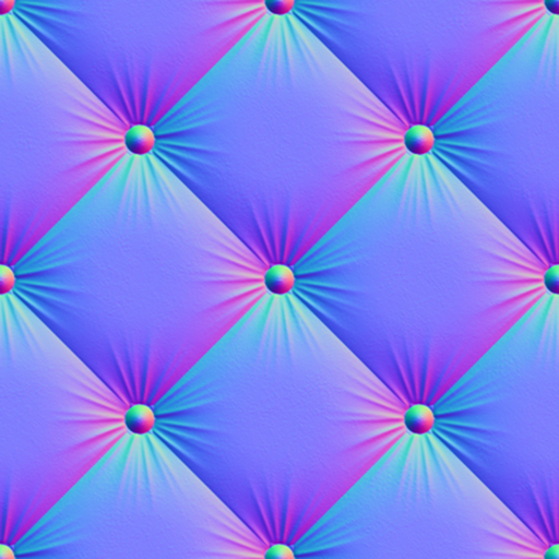
After we calculate the tangent and bitangent vectors, we can use these vectors to transform the normal values from the textures to the tangent space. Below you can see a normal map of a cushion, and the values are close to blue, which you can see on the normal maps frequently. The reaseon behind it is that the normal maps are in tangent space which is defined with Tangent, Bitangent and Normal vectors respectively. And the normal maps tends to not change the normals too much to prevent causing visual artifacts, which makes the normal maps to be close to blue.
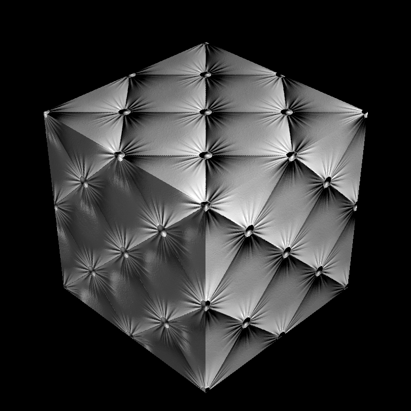
Normal map applied to a cube
Normal map applied to a cube
Normal map applied to a sphere
Normal map applied to a cube
Normal map applied to a cube
Bump Mapping
The normal mapping method is not the only method to create more detailed models. We can use the bump mapping method to create more detailed models. The bump mapping method is similar to the normal mapping method, however, instead of using the normal values from the textures, we can use the height values from the textures to create more detailed models. To do so, we can just sample the height values from the textures and use them to create a new intersection point which is displaced from the original intersection point. After that we can use this new intersection point to calculate the normal values of the intersection point. To do so, we can just use the partial derivatives of the height values to calculate the tangent and bitangent vectors of the intersection point. To calculate the partial derivates with the displaced point we can use the chain rule. After that we can use these vectors to calculate the normal values of the intersection point.
To calculate the partial derivatives of the height values, we can use the following code snippet.
color bump_bottom, bump_left, bump_top, bump_right;
rec.mat_ptr->bump_map->area_values(uv.x(), uv.y(), rec.p, bump_top, bump_bottom, bump_left, bump_right);

float l0 = bump_value.luminance();
float l1 = bump_right.luminance();
float l2 = bump_top.luminance();

rec.p = rec.p  + rec.normal * l0 * rec.mat_ptr->bump_factor;

auto delu = 1.0f / (float)rec.mat_ptr->bump_map->width;
auto delv = 1.0f / (float)rec.mat_ptr->bump_map->height;

auto dqdu = tangent + ((l1 - l0)) * rec.mat_ptr->bump_factor * normal / delu;
auto dqdv = bitangent + (k * (l2 - l0)) * rec.mat_ptr->bump_factor * normal / delv;

rec.normal = unit(cross(dqdv, dqdu));
This calculation gave results that are looking bumpy, however the results are noticably more bumpier than the reference images, I tried to fix this by halving the uminance values I sampled from the image however, the results are still off. In the end, I reverted this change to be more consistent with my implementation.
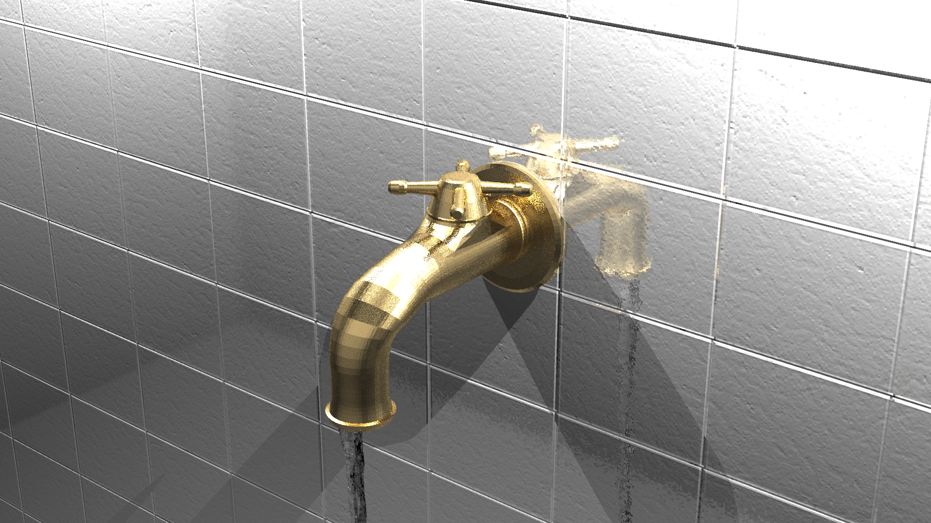
Earth texture mapped onto a sphere with bump values
Earth texture mapped onto a sphere with bump values

Wood texture mapped onto a cube with bump values
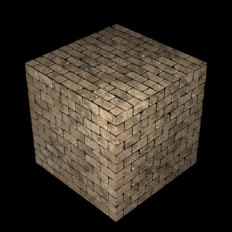
Wall texture mapped onto a cube with bump values
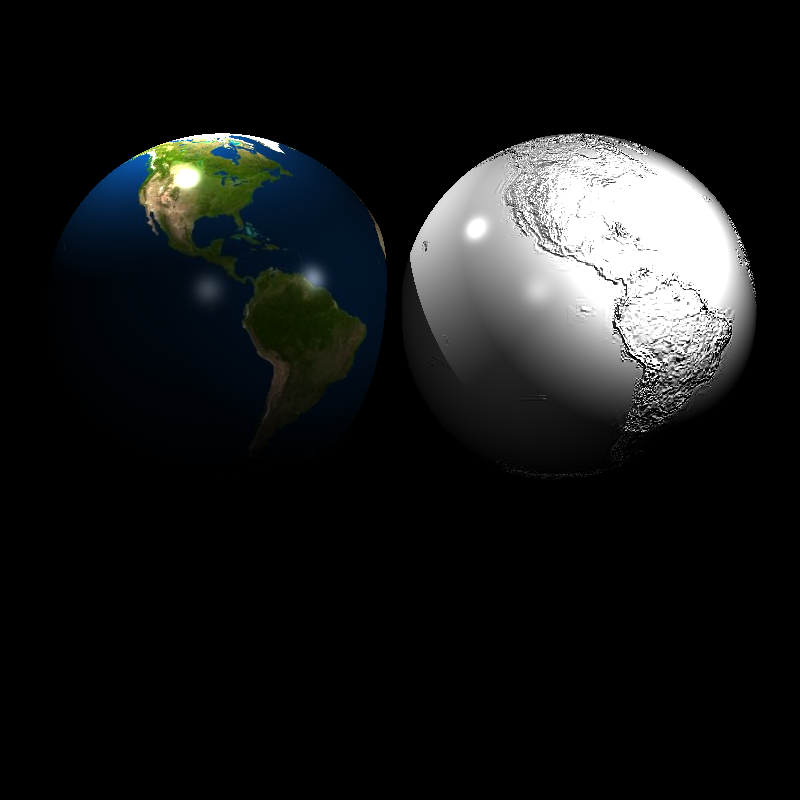
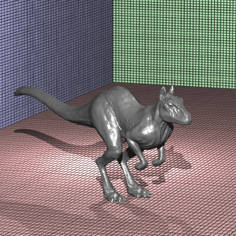
Bump mapping applied to a spaceship with motion blur
Bump mapping applied to a transformed model
Bump mapping applied to a transformed model
Perlin Noise
To create procedural effects we can create textures with perlin noise. Perlin noise is a type of gradient noise which is created by interpolating random values from the 3D points, which will have continuity and consistent results. I won’t go into the details of the perlin noise (you can see the details from one of my older posts in which I create a terrain using perlin noise with geometry shaders), however, I will show how to apply bump mapping with perlin noise using surface gradients. To do so we just need to calculate the gradient of the perlin texture on the given point and use it to calculate the normal values of the intersection point. Below you can see the results of the perlin noise bump mapping.
auto pv = perlin_texture->value(rec.uv.x(), rec.uv.y(), rec.p).x();

float eps = 0.0001f;
auto dx = perlin_texture->value(rec.uv.x(), rec.uv.y(), rec.p + vec3(eps, 0, 0)) - perlin_texture->value(rec.uv.x(), rec.uv.y(), rec.p);
auto dy = perlin_texture->value(rec.uv.x(), rec.uv.y(), rec.p + vec3(0, eps, 0)) - perlin_texture->value(rec.uv.x(), rec.uv.y(), rec.p);
auto dz = perlin_texture->value(rec.uv.x(), rec.uv.y(), rec.p + vec3(0, 0, eps)) - perlin_texture->value(rec.uv.x(), rec.uv.y(), rec.p);

auto gradient = vec3(dx.x(), dy.x(), dz.x()) / eps;
auto g2 = dot(gradient, normal) * normal;
auto g1 = gradient - g2;

rec.normal = unit(normal - g1);
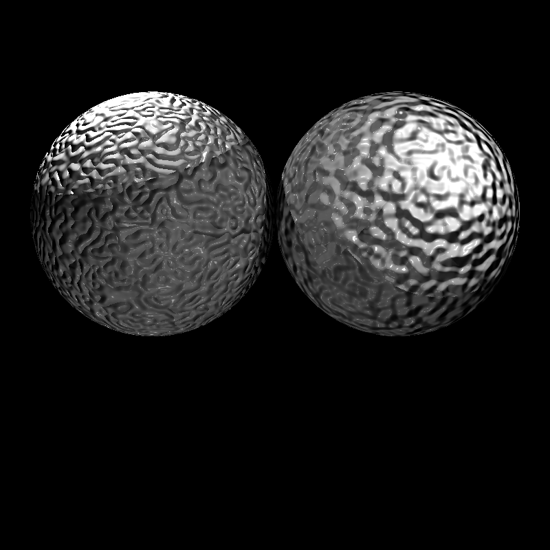
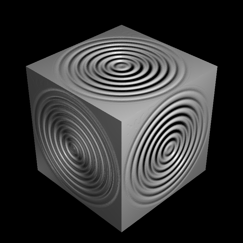
Perlin noise bump mapping applied to a sphere
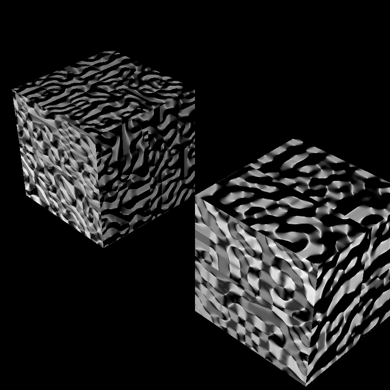
Perlin noise bump mapping applied to a cube
And we can use the perlin noise directly as color values as seen bleow.

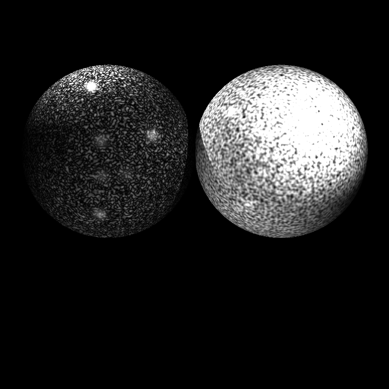
Perlin noise applied to a sphere
Perlin noise applied to a sphere with scale
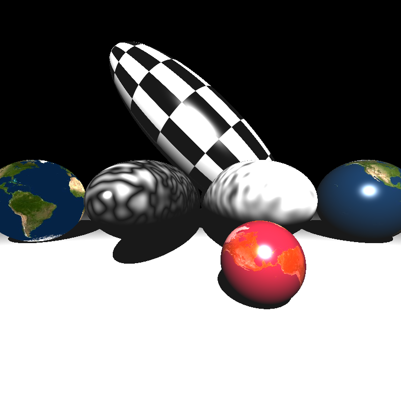
Different textures applied to a bunch of ellipsoids
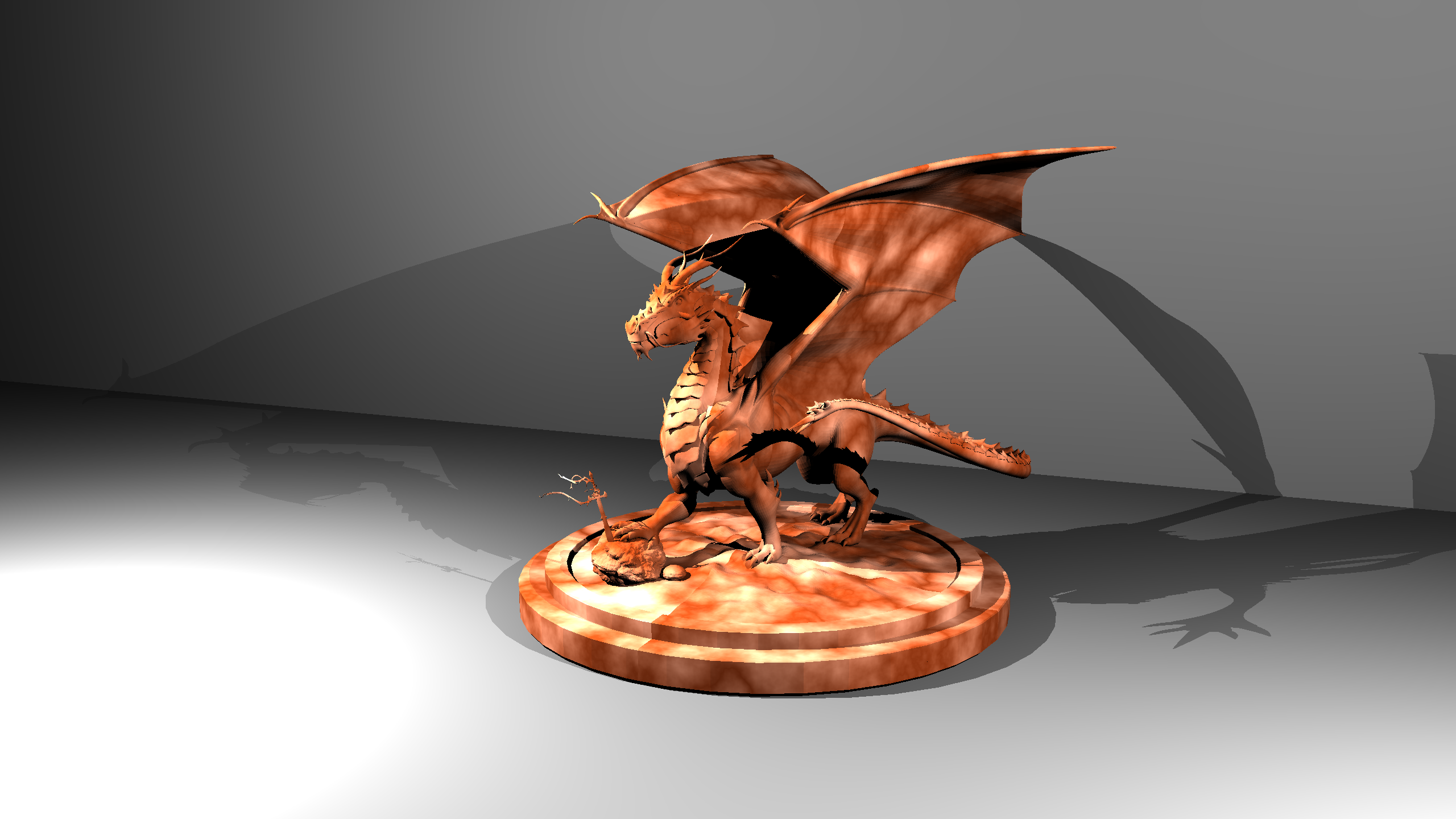
Perlin noise applied to a dragon model
References
Ahmet Oğuz Akyüz, Lecture Slides from CENG795 Advanced Ray Tracing, Middle East Technical University