With our CPU ray tracer in our hand, we can handle multiple materials and create some beautiful images. However, the process is slow, and we can optimize many things in our code. In this post, we will optimize our ray tracer with acceleration structures, tiled multithreading and some linearization.
Bounding Volume Hierarchy
In our ray tracer, we need to check every object in the scene to find the closest intersection point. This process is slow, especially when we have many objects, like millions of triangles, in the scene. To speed up this process, we can use a Bounding Volume Hierarchy (BVH) structure. BVH is a tree structure that divides the scene into volumes and stores the objects in these volumes. With this structure, we can check the intersection with the volumes first, and if the ray intersects with the volume, we can check the objects in that volume. This way, we can reduce the number of intersection checks and speed up the process.
First, I thought implementing a basic BVH with nodes that have pointers in them pointing other nodes or objects. However, this approach is not cache-friendly and can be slow. I looked into the linear versions of BVH and seemed simple enough to create it from the scratch. First, I created the node structure to hold the bounding box and the children nodes, and for the leaf nodes we need to have the object positions in the respected structure.
struct BVHNode
{
	vec3 aabb_min, aabb_max;
	uint32_t left_child;
	uint32_t first, count;
	bool is_leaf() const { return count > 0; }
};
At first, I thought having the right child index and a bool to hold the leaf status would be enough. However, I realized that I only need to have the left child index, and then while traversing the tree I can calculate the right child index with the placements I made while building the BVH. And for the leaf nodes, I can use the count variable to hold the number of objects in the leaf node, and if the child count is zero, then it is not a leaf node, because In BVH, only the leaf nodes have triangles in them. This made my node structure 36 bytes, which is a good size for cache-friendly operations.
After creating the BVH structure, I needed to build the BVH. To build the BVH, as a first step, I calculated the centroids of the triangles and to split each node, I used a basic split mode which halves the most extended axis of the bounding box. After the split, I created the left and right child nodes and assigned the triangles to the respected child nodes. I repeated this process until I reached the leaf node.
And voila, I have a BVH structure that can handle the scene with millions of triangles. For testing, I used the Dragon model which has 869928 triangles, and the BVH structure handled it like a charm.
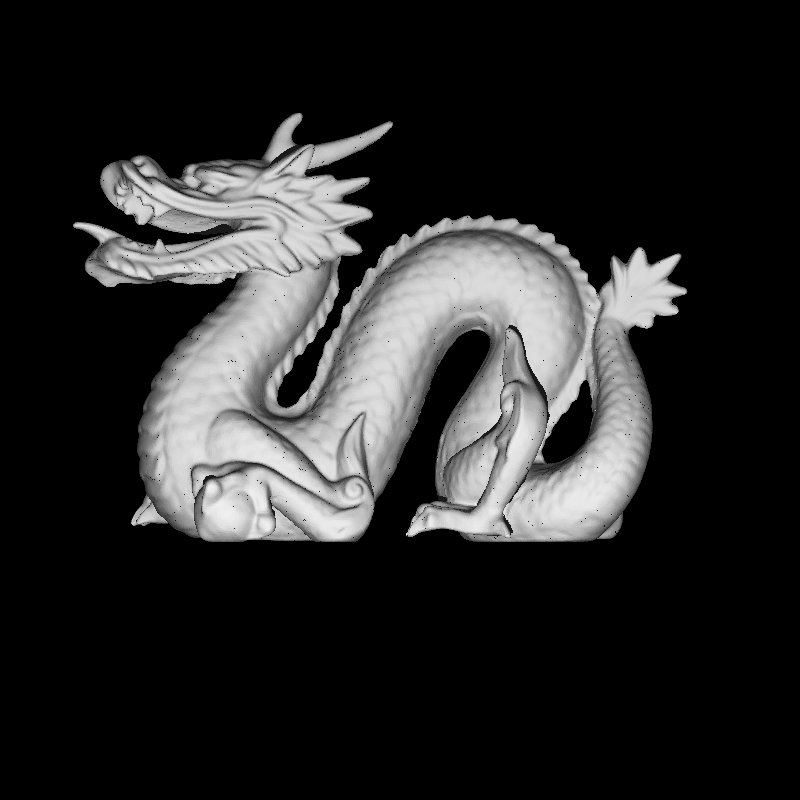
Dragon model with BVH structure rendered in 789ms
Before the BVH structure, the same scene was rendered in 15-20 mins. This is a huge improvement, like 20x faster.
However, while implementing the BVH structure, I realized that there are some black artifacts present in the image. At first, I thought that BVH structure is causing this, however the issue was the intersection code. I implemented the Möller–Trumbore intersection algorithm, I tried to adjust the epsilon values to fix the issue, it did help decrease the artifacts, however, it did not eliminate them. To solve this issue, I jumped back to the barycentric coordinates method, and adjusts the epsilons accordingly, and the artifacts were gone. And to my surprise, the barycentric coordinates method was faster than the Möller–Trumbore algorithm, at least in my implementation.

Dragon model without artifacts in 730ms
Tiled Multithreading
There is an indeed huge speedup with the BVH structure, however, we can still optimize the process. In the previous post, I mentioned that I used a simple multithreading approach. While examining the code, I realized that I spawned a thread for each pixel (I used std::future and async, and I believe behind the scenes It doesn’t use a thread pool). To fix this issue, I implemented a basic thread pool, in which each thread gets the jobs from a job queue until there is no job left in the queue. Which ensures that no thread is waiting for a job after finishing the previous one, if we enqueue jobs fast enough. While doing the pooled multithreading, I also implemented a tiled multithreading approach. In this approach, I divided the image into 32x32 tiles, and enqueued each tile as a job into the pool. While testing the structure I came across a deadlock which prevented the threads getting new jobs as they are not notified when a job is available if we wait all the threads to finish. I solved this issue by adding a second conditional variable. The results were satisfying, for the dragon model I can render the scene in 60ms, which is a huge improvement in addition to the BVH structure. In the end, we decreased the render time from 15-20 mins to 60ms. The job loop for the thread pool is below:
    ThreadPool(size_t threads) {
        for(size_t i = 0; i < threads; ++i) {
            workers.emplace_back([this] {
                while(true) {
                    std::function<void()> task;
                    {
                        std::unique_lock<std::mutex> lock(queue_mutex);
                        task_condition.wait(lock, [this] {
                            return stop || !tasks.empty();
                        });

                        if(stop && tasks.empty()) {
                            return;
                        }

                        task = std::move(tasks.front());
                        tasks.pop();
                    }

                    active_tasks++;
                    task();

                    {
                        std::unique_lock<std::mutex> lock(queue_mutex);
                        active_tasks--;
                    }
                    finished_condition.notify_all();
                }
            });
        }
    }
Instancing and Transformations
If we have a fast ray tracer with a BVH structure, we can push the limits and have multiple of these huge models. And in fact, if we want to have multiple of the same model, we can cut from the memory cost by using instancing. We can just store each base model once in our memory and after that we can just reference the base model for other instances. However, to have meaningful renders, we need to move them around, rotate them, and scale them. To do this, we can implment transformations and apply them to the instances. For the transformations, I implemented a 4x4 matrix structure and converted each transformation into the matrix equivalent.
To implmement instancing to our BVH structure, I created a new structure called BVHInstance to reference the base model’s BVH structure, the transformation matrix and the material information.
struct BVHInstance : public hittable
{
	std::shared_ptr<BVH> bvh;
	std::shared_ptr<material> mat_ptr;

	BVHInstance(std::shared_ptr<BVH> _bvh) : bvh(_bvh) {}
	BVHInstance(std::shared_ptr<BVH> _bvh, mat4 _model) : bvh(_bvh) { model = _model; }

	bool hit(const ray& r, double tMin, double tMax, hitRecord& rec, mat4* model) const override;
};
Hitting Transformed Instances
These instances are nice and can be created easily, but our camera spawns rays in the world space, and we need to transform these rays into the object space to check the intersections. To do this, we can use the inverse of the transformation matrix. We need to transform the ray’s origin and direction, with respect to this inverse matrix. For a small note, we need to add 4th elements to the ray’s origin and direction to make the matrix multiplication work with the 4x4 matrix. This is a common practice in computer graphics, and it is called homogenous coordinates. We add 0 as the 4th element for the direction and 1 for the points, because the directions do not need to be translated, only the points need to be translated, which we calculate our matrices accordingly.
auto invModel = object->model.inverse();
ray newRay = r;
vec4 origin = vec4(newRay.origin(), 1.0f);
vec4 direction = vec4(newRay.direction(), 0.0f);

vec4 newOrigin = invModel * origin;
vec4 newDirection = invModel * direction;

newRay = ray(vec3(newOrigin.x(), newOrigin.y(), newOrigin.z()),
             vec3(newDirection.x(), newDirection.y(), newDirection.z()));
After this implementation, we can have multiple instances of the same model with different transformations and materials.

9 Dragon instances rendered in 1188ms
Issue with Normals
While implementing the transformations, I realized that the normals are not transformed correctly. At first, I thought that the normal transformation calculations are the suspect, (we transform normal values with respect to the inverse transpose of the model matrix), but this was not the case. In the previous iteration, I calculated the normals in the hit function of the objects, and if the normal does not face the ray direction, I negated it, and made the refraction calculations based on this assumption. I believe, this model has some planar surfaces, and the normal calculations are not correct for these surfaces. To fix this issue, I calculated the normals in the intersection functions of the objects, and I did not negate the normals. And for the refracted materials, I negated the normals if it is a backface.
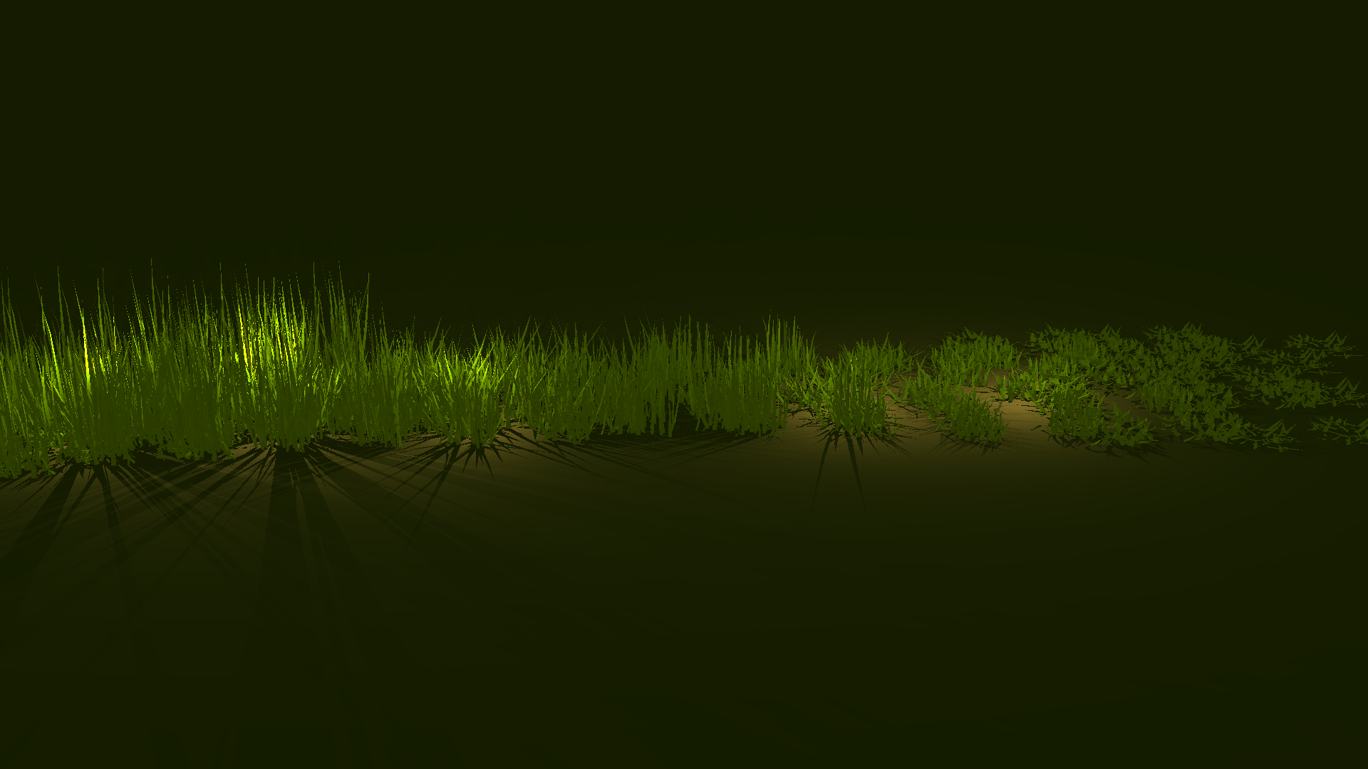
Faulty normals of the grass

Correct version of the normals rendered in 6679ms
Back to the BVH, is a better split possible?
While testing the BVH structure, some scenes, didn’t render as fast as I expected. While experimenting with some stuff on the code, I noticed that some leaf nodes didn’t split any triangles, and have all the triangles in one child which can have like 240 triangles which is bad. To solve this issue I tried to split the triangles equally, for each axis, I tried different split points and calculated the cost of the split. I used a very basic cost function, which is the count difference between the nodes after we split them. Then I used the minimun cost split point for the split. This approach worked well, and the render times decreased for some meshes. However, for some meshes like the dragon model, the render time increased. I believe this is the result of my cost functions, it can work well for meshes with longer triangles, however bad for meshes with shorter and smaller triangles. I am not exactly sure this is the cause, it is just a guess and needs further investigation.
For the windmill scene, it worked well, and the render time decreased from 1080ms to 484ms.

Windmill scene rendered with a better split in 484ms, 2x faster than the basic split method
Too Many BVHs, Time For a BVH of BVHs Also Known As Top Level Acceleration Structures
In the previous windmill scene, there are 20 meshes to render, and each mesh has its own BVH structure. And our rays won’t intersect with many of them, in this case we don’t have many meshes, but we still can reduce the number of intersection checks. To do this, we can create a top-level BVH structure, which holds the BVH structures of the meshes. We can check the intersection with the top-level BVH first, then with the BVH structures of the meshes. However, there is a catch, we need to transform the bounding boxes of these BVH structures with respect to their model matrices and move them into the word space to correctly build the top level BVH structure. I used the same building method and split function to build the top-level BVH structure, the main difference is that leaf nodes hold the BVH structures of the meshes.
The results for the windmill scene were satisfying, the render time decreased from 484ms to 419ms. However, for the grass scene this approach increased the render time from 6679ms to 7226ms. I believe this is the result of the additional intersections with bounding boxes, which can be unnecessary for some scenes. I believe this approach can be useful for scenes with many meshes, and for scenes with a few meshes, it can be slower than the basic BVH structure.

Windmill scene rendered with a TLAS BVH in 419ms
Timings with Different Approaches
| Scene | Half Split BVH Tiled MP | Experimental Split BVH Tiled MP | Half Split TLAS BVH Tiled MP | Experimental Split TLAS BVH Tiled MP | Experimental Split BVH Basic MP |
|---|---|---|---|---|---|
| Dragon | 84ms | 363ms | 90ms | 375ms | 1051ms |
| Glaring Davids | 283ms | 748ms | 222ms | 757ms | 1324ms |
| Lobster | 837ms | 2211ms | 893ms | 2274ms | 3510ms |
| Science Tree | 145ms | 157ms | 157ms | 173ms | 1179ms |
| Ton Roosendaal | 73ms | 68ms | 84ms | 76ms | 312ms |
| Dragon Metal | 1225ms | 8773ms | 1315ms | 7327ms | 9803ms |
| Ellipsoids | 101ms | 103ms | 1086ms | 112ms | 744ms |
| Marching Dragons | 1227ms | 3655ms | 1230ms | 3673ms | 5699ms |
| Metal Glass Plates | 632ms | 747ms | 639ms | 688ms | 1163ms |
| Simple Transform | 46ms | 44ms | 45ms | 47ms | 741ms |
| Spheres | 87ms | 90ms | 106ms | 104ms | 726ms |
| Two Berserkers | 364ms | 357ms | 210ms | 130ms | 993ms |
| Windmill | 1158ms | 483ms | 961ms | 444ms | 1034ms |
| Grass Desert | 6930ms | 7886ms | 7330ms | 8512ms | 10097ms |
Result Images and Videos
The results of transformed lights, transformed cameras, transformed and instanced models can be seen below as images and videos.

Chinese Dragon
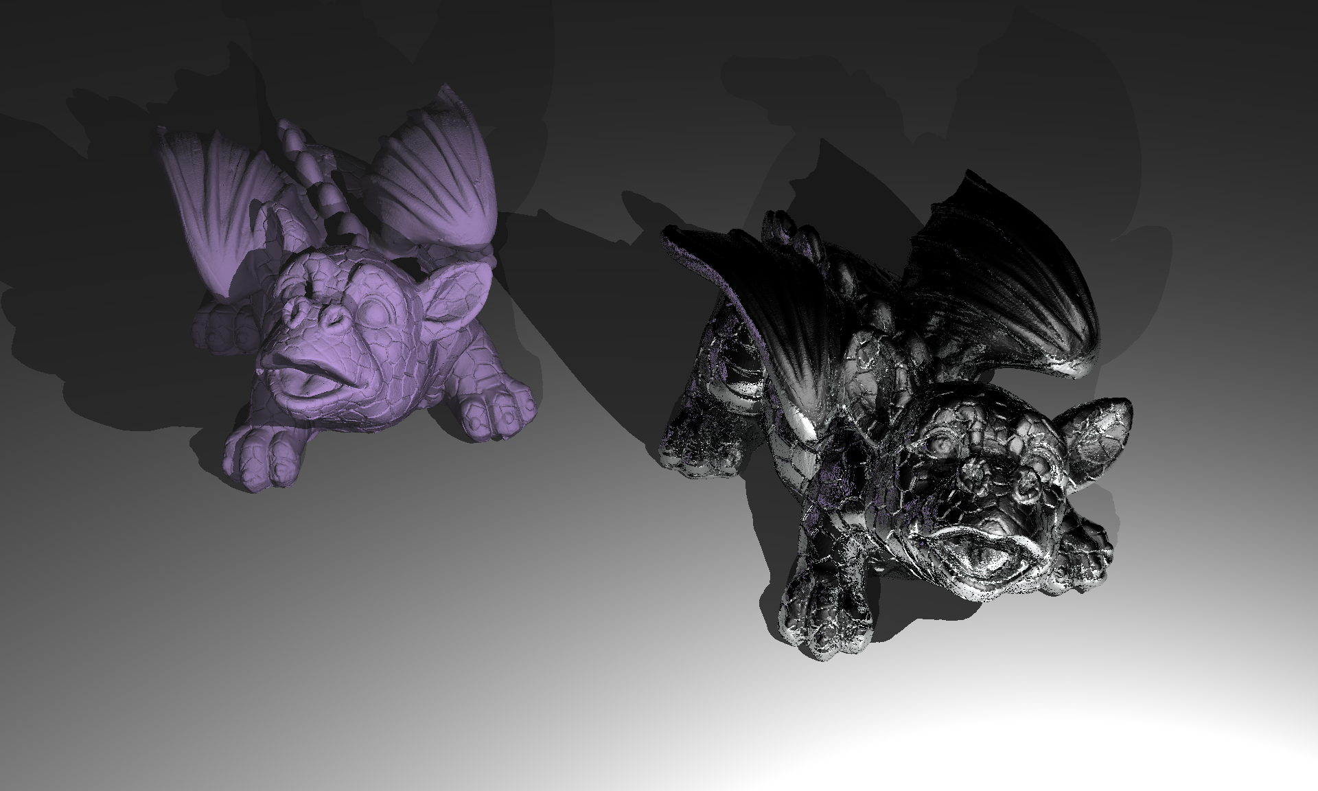
Metal Dragon
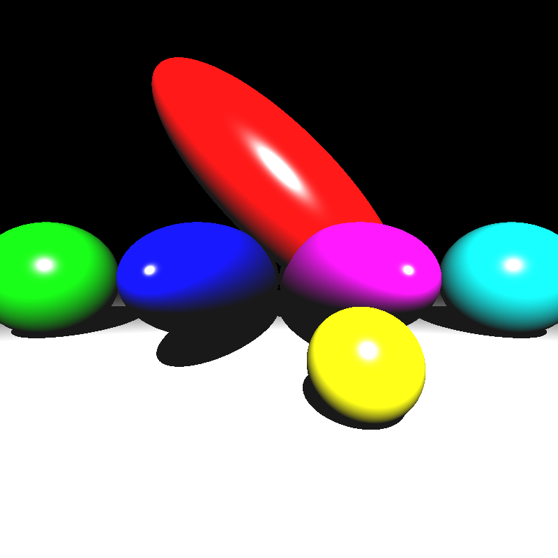
Ellipsoids
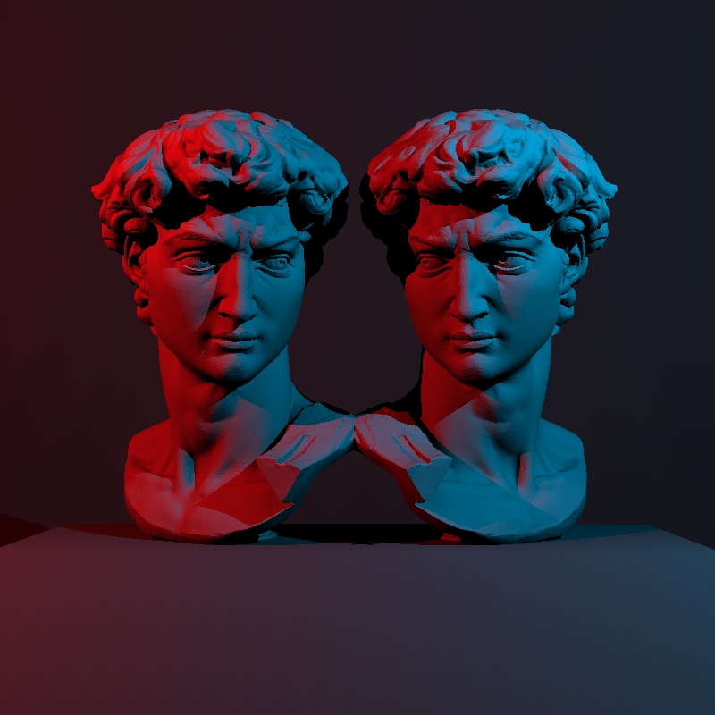
Glaring Davids
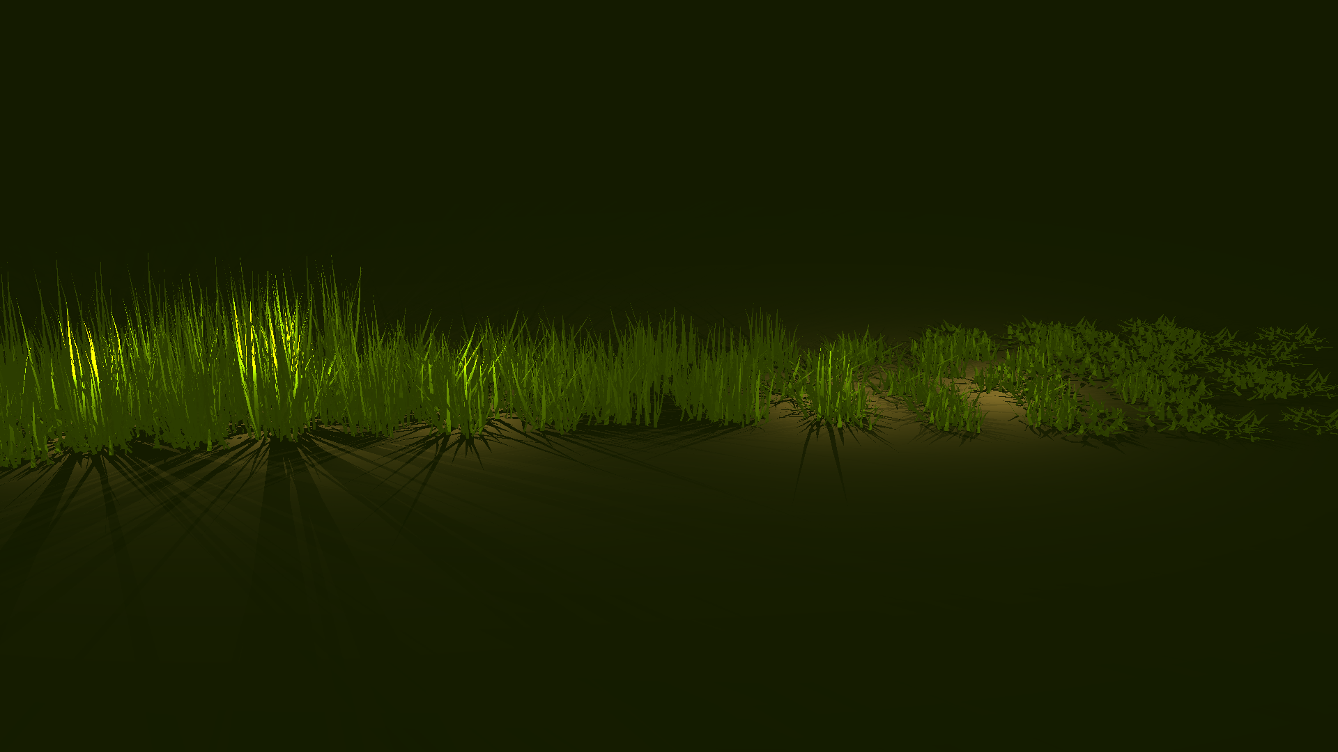
Grass Desert
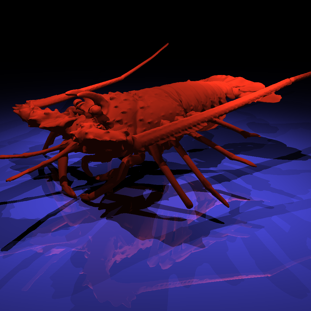
Lobster
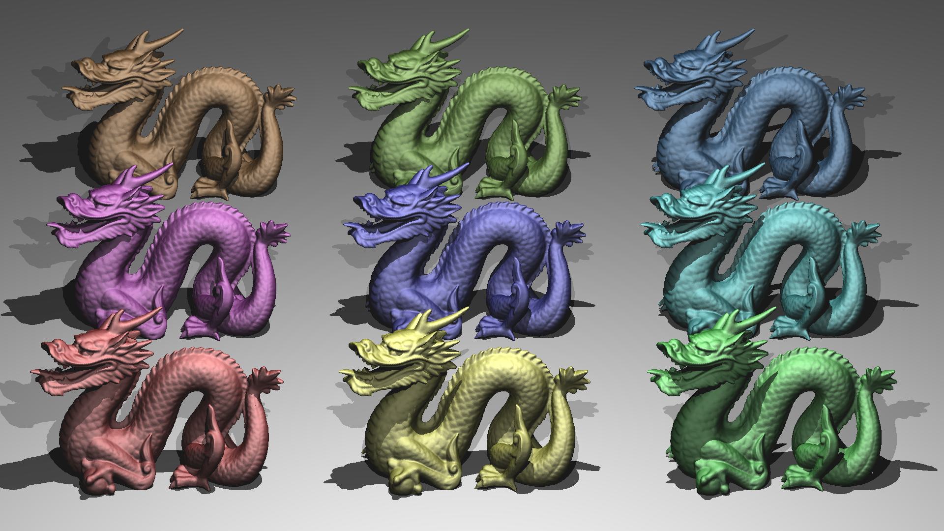
Marching Dragons
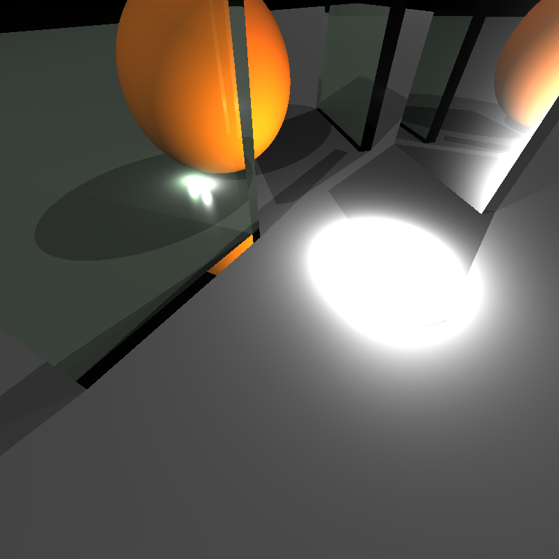
Metal Glass Plates
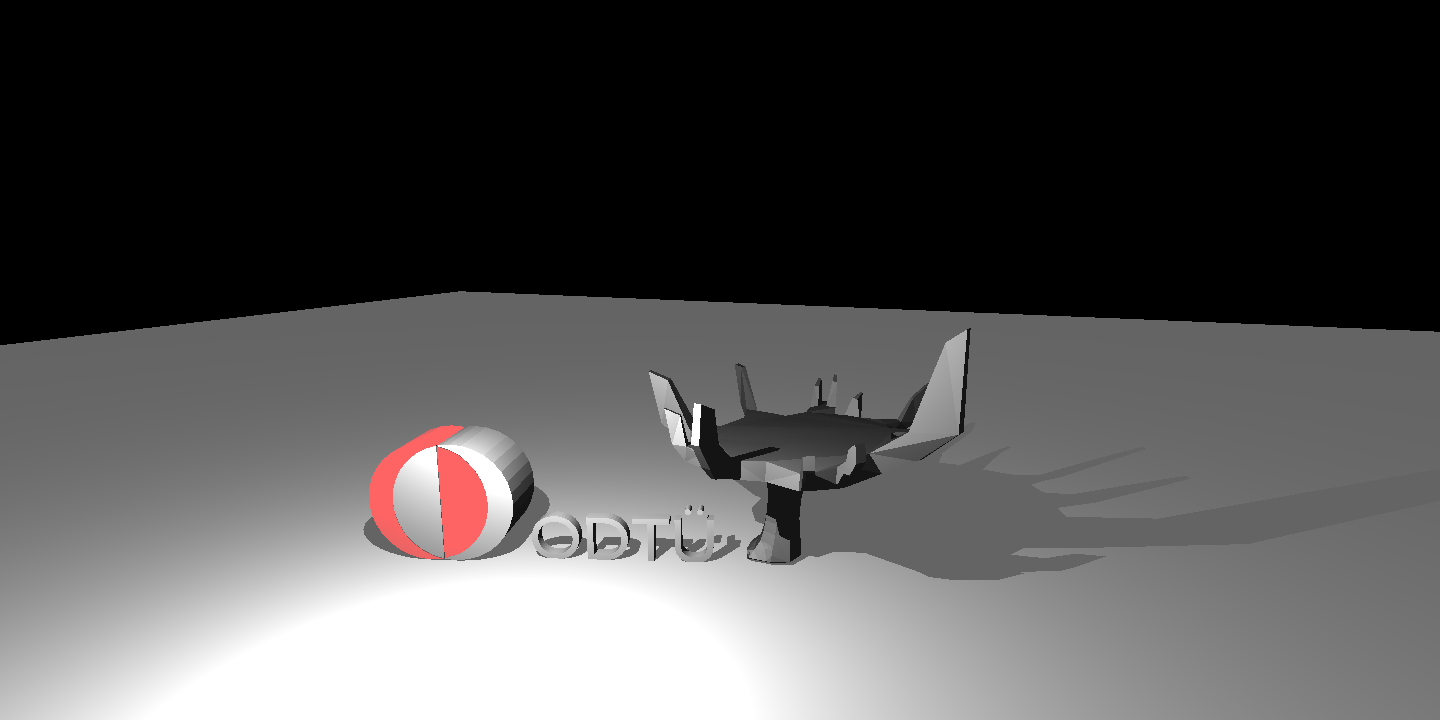
Science Tree
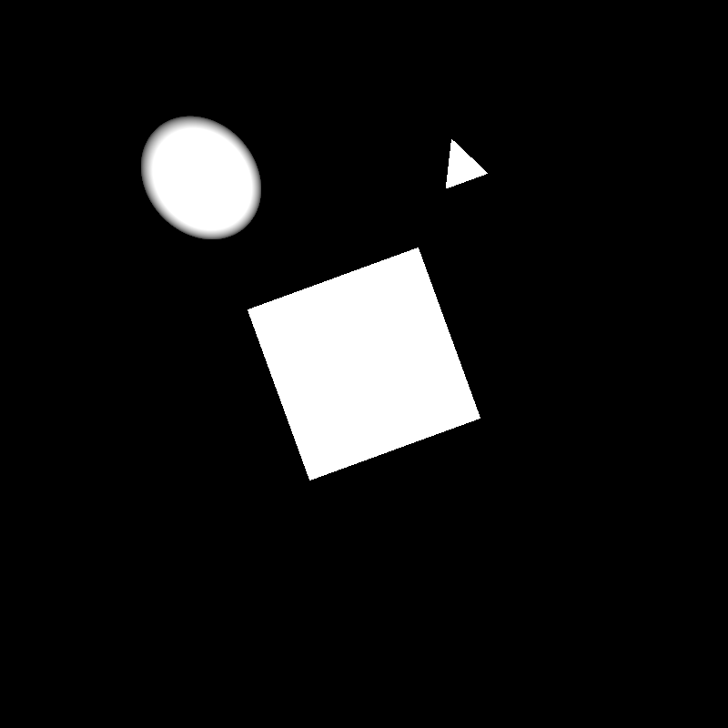
Simple Transform
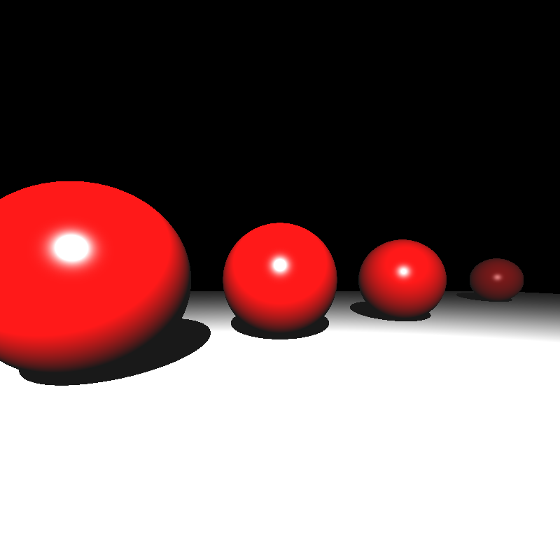
Spheres
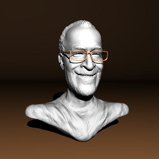
Ton Roosendaal
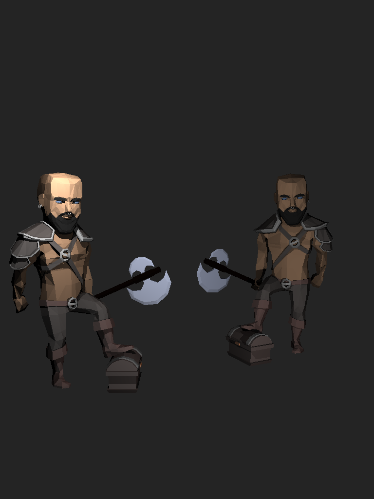
Two Berserkers
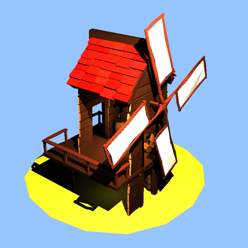
Windmill
References
“Jacco Bikker,. How to build a BVH.” https://jacco.ompf2.com/2022/04/13/how-to-build-a-bvh-part-1-basics
Ahmet Oğuz Akyüz, Lecture Slides from CENG795 Advanced Ray Tracing, Middle East Technical University